
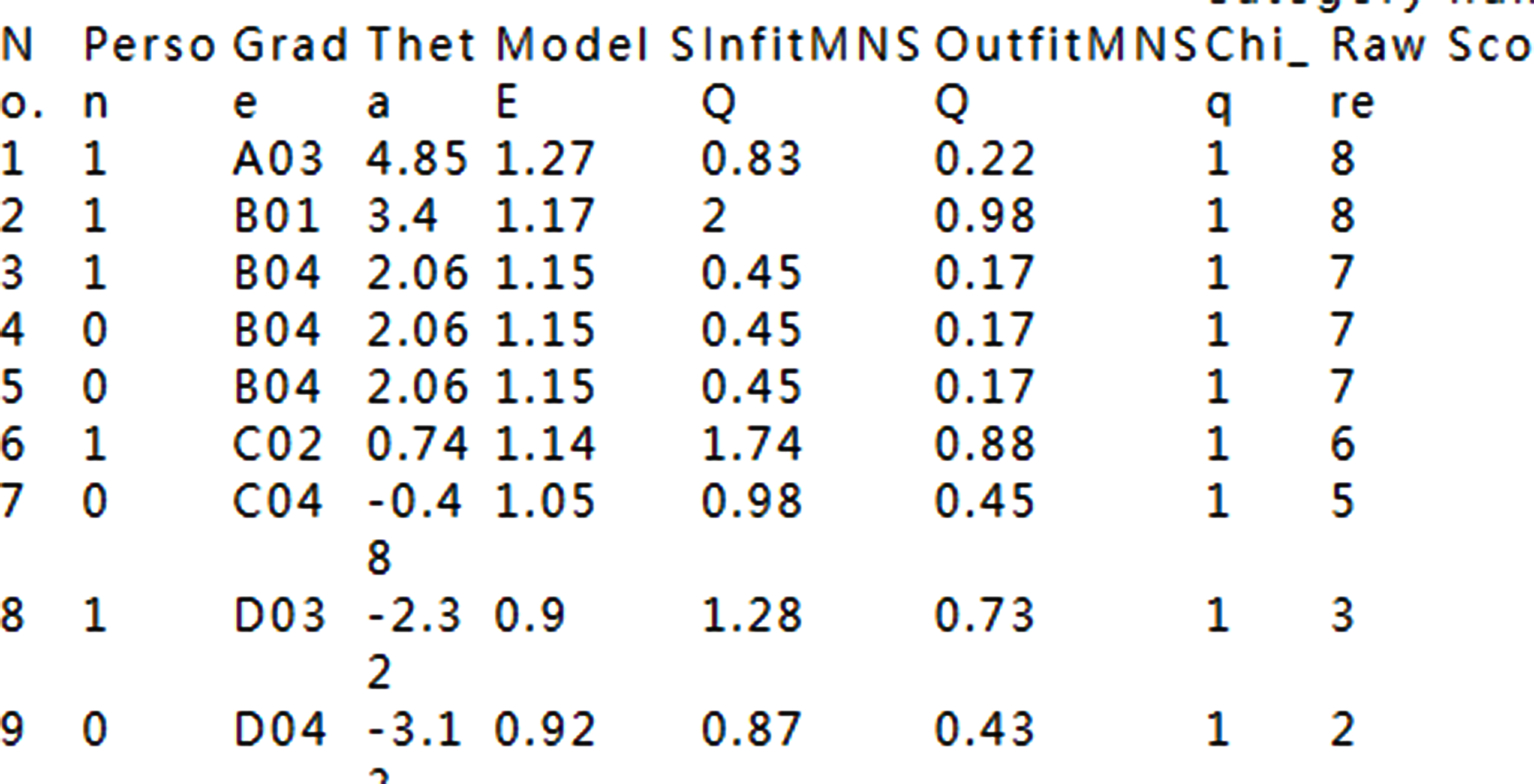
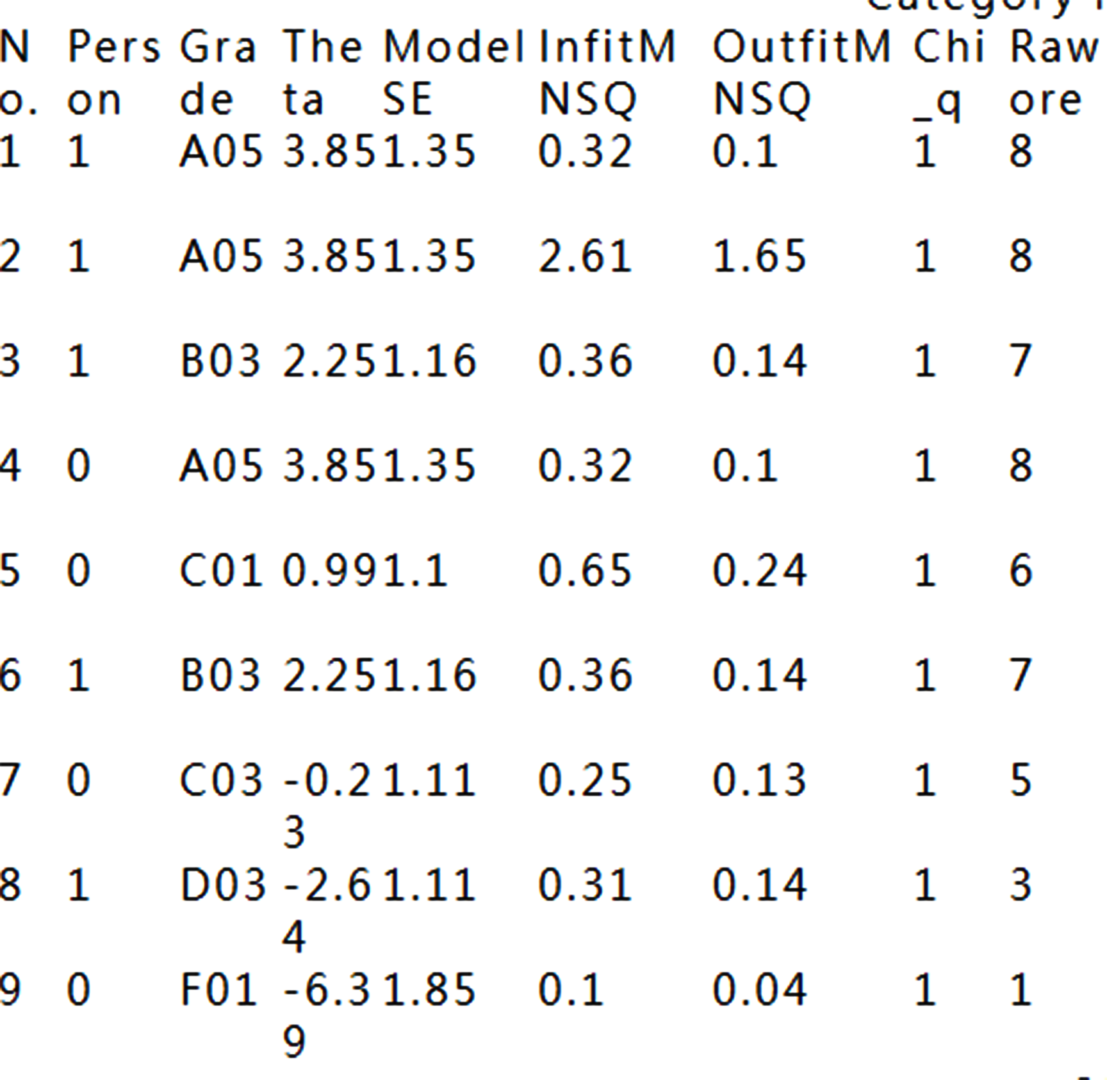
A03 means the ability with measures at the top, followed by B, C, and D grades.
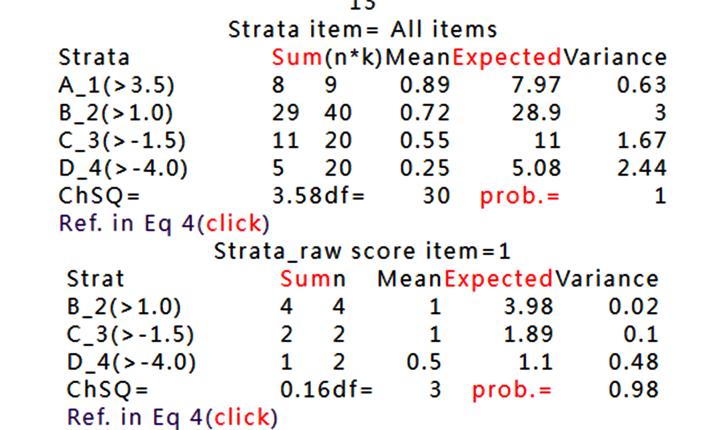
That is, four strata from A to D are divided in this dataset.
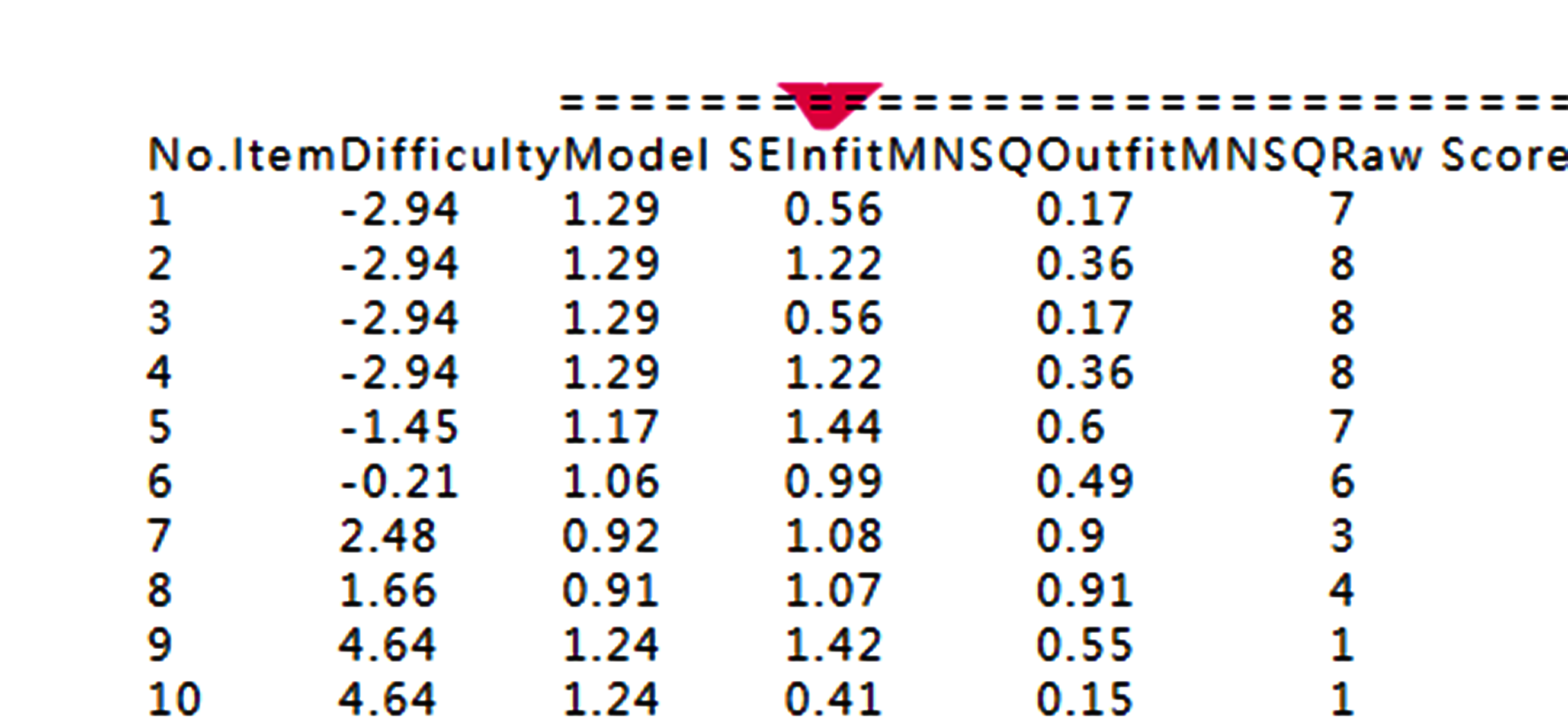
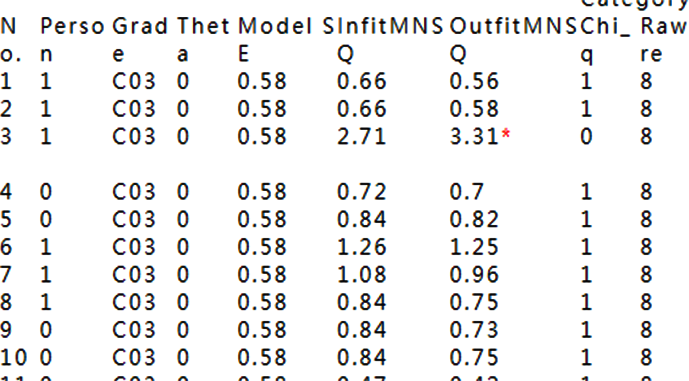
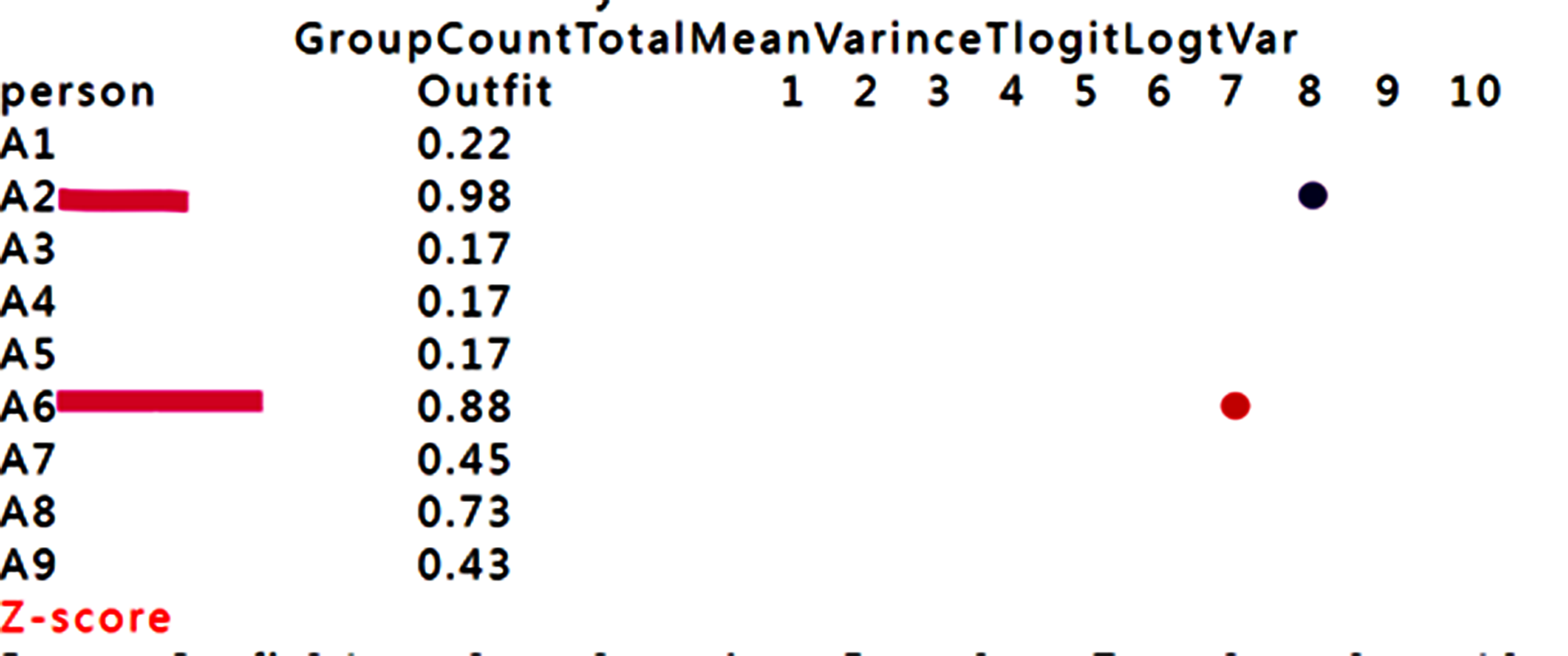
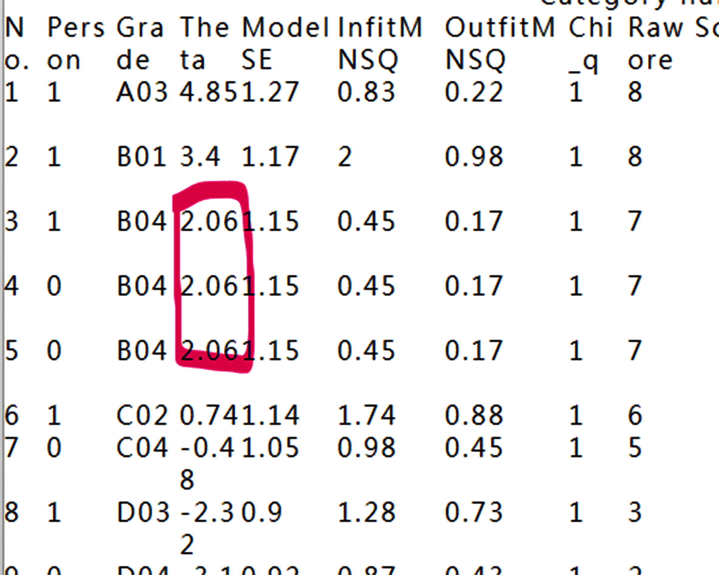
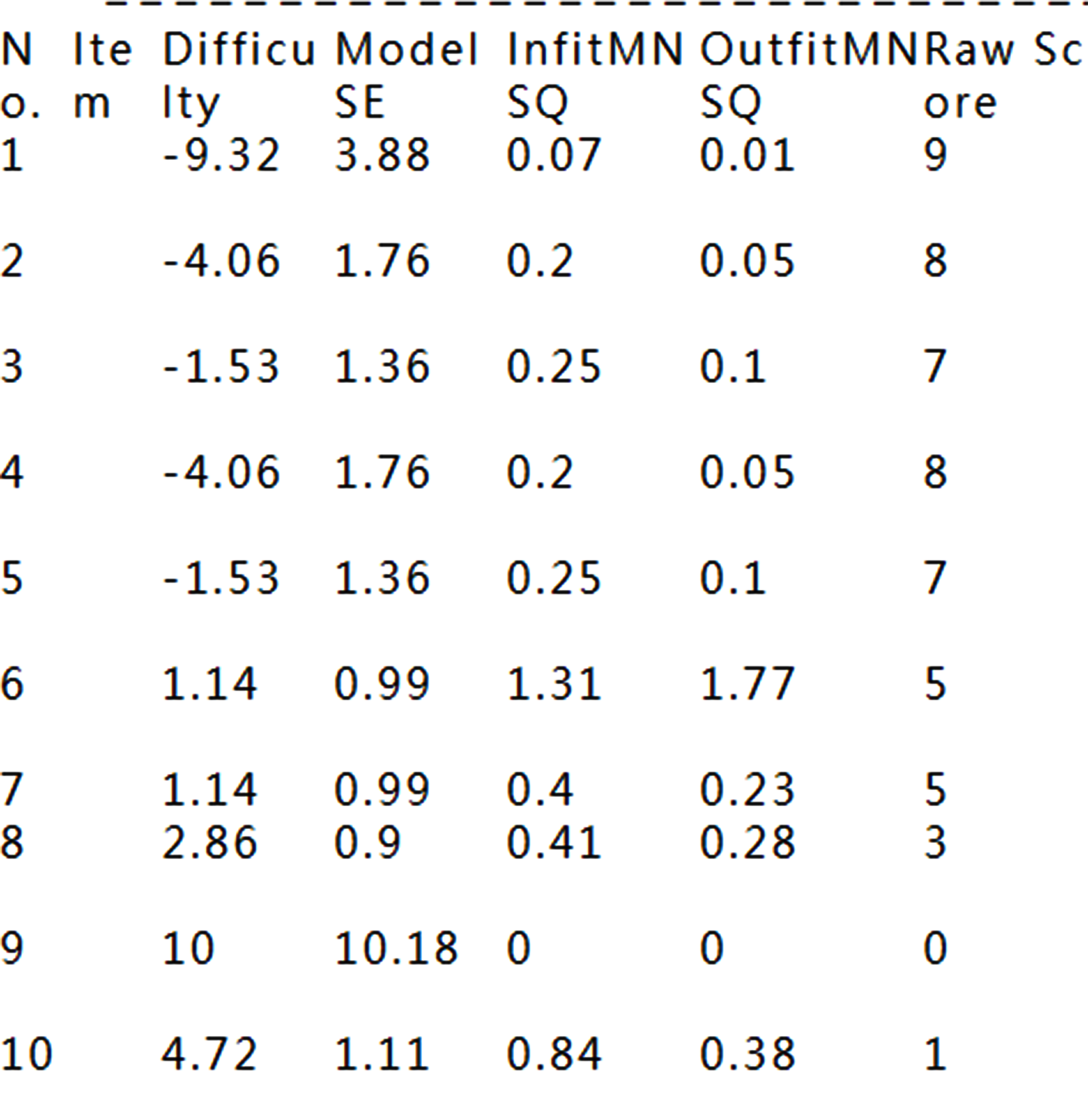
Item difficulties are listed with measures, SE, Infit and Outfit MNSQs. The correlation coefficient between raw scores and item difficulties is negative. A high raw score has a lower item difficulty.
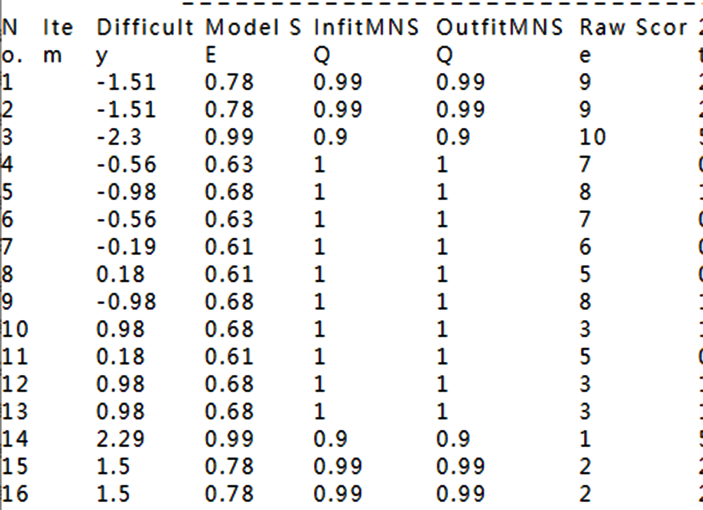
Item difficulties are listed with measures, SE, Infit and Outfit MNSQs. The correlation coefficient between raw scores and item difficulties is negative. A high raw score has a lower item difficulty.
2.Summary Table
If the summary table is selected, the results are shown below:
2.Summary Table
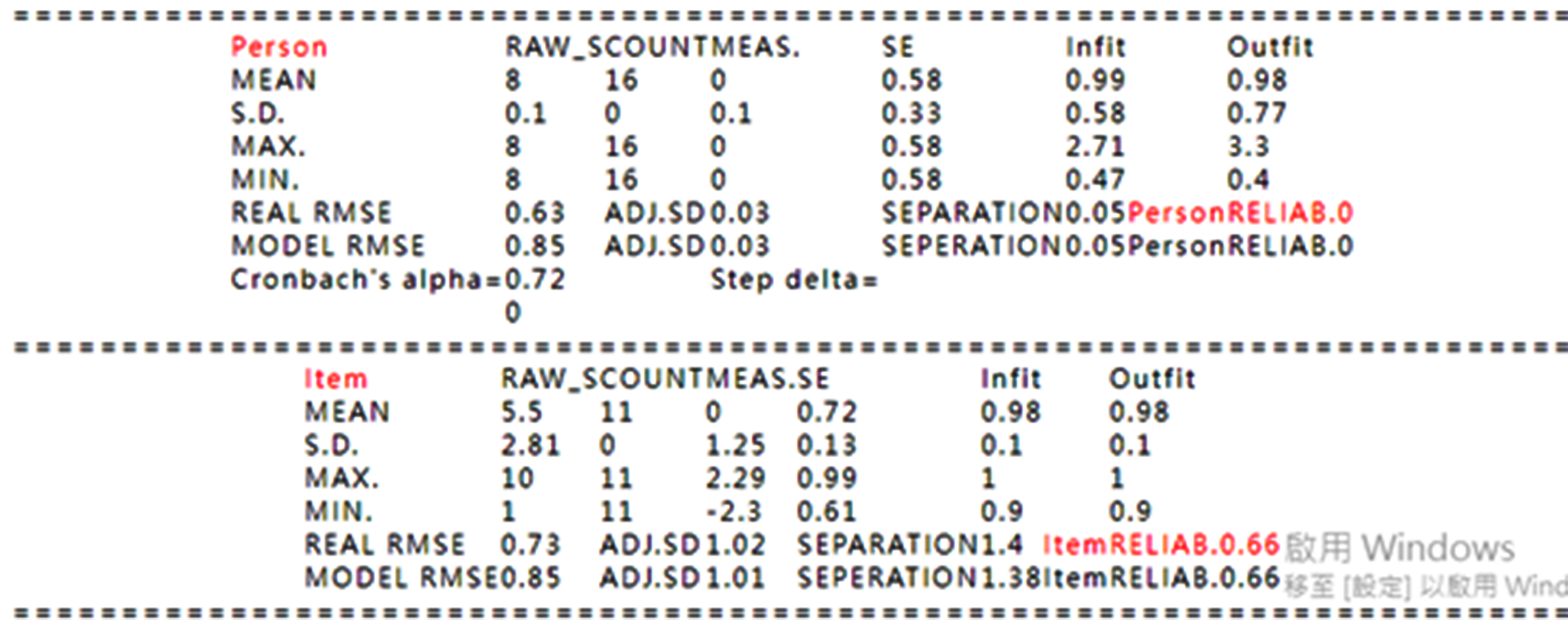
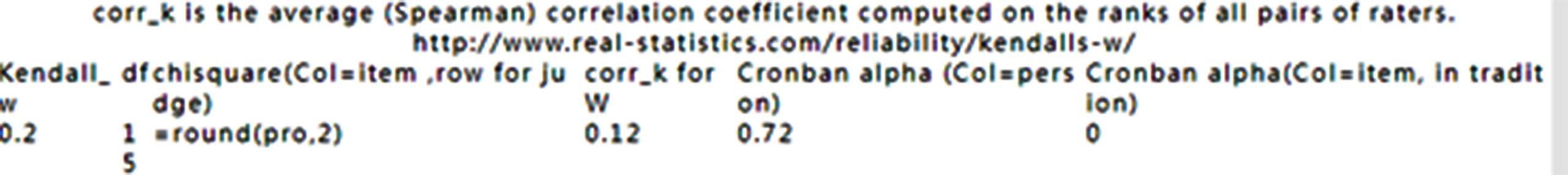
Person reliability (top) and item reliability(bottom) are shown at the bottom right, with values of 0 and 0.66, respectively. Note that the reliability is Rasch reliability rather than the Cronban’s alpha shown in the previous section.
(It is worth learning how to compute those values in the Table of person and item parameters. Any further information is to read relevant references in Rasch analysis or refers to Winsteps Manual for readers.
3.Overall Fit Stat.
Model data fit with the method separating several strata in measure and examining counts in difference between expected and observed occurances among stratra.
2.Summary Table
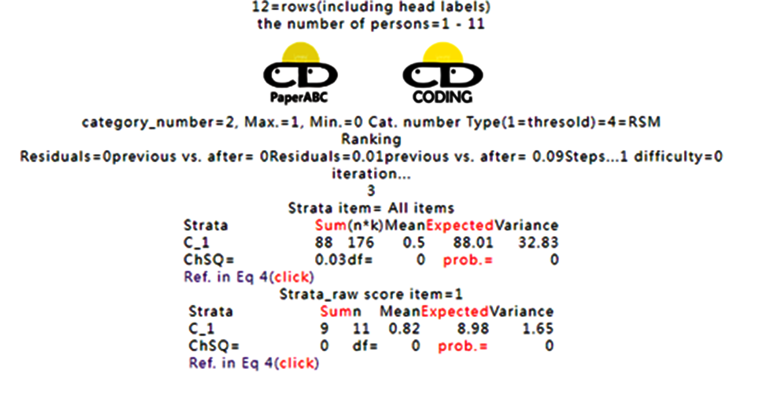
Ten rows exist in this dataset with the maximum=1 and nine persons
The number of categories is 2 with maximum=1 and minimum=0 under the rating scale model(RSM)
Model residual stops at 0.05. Due to the dichotomous responses, the step threshold is one and the mean difficulty as usual is set at zero.
Iteration numbers=13
Four strata are in existence. The model data fit is expressed by chSQ=3.58 with df=30 and prob.=1.0, indicating the data fit the Rasch model fairly well.
Note that if the fit statistics with Infit MNSQ are shown later in this manual, we can see that all items’ Infit MNSQs are within the criteria between 0.5 and 1.5.
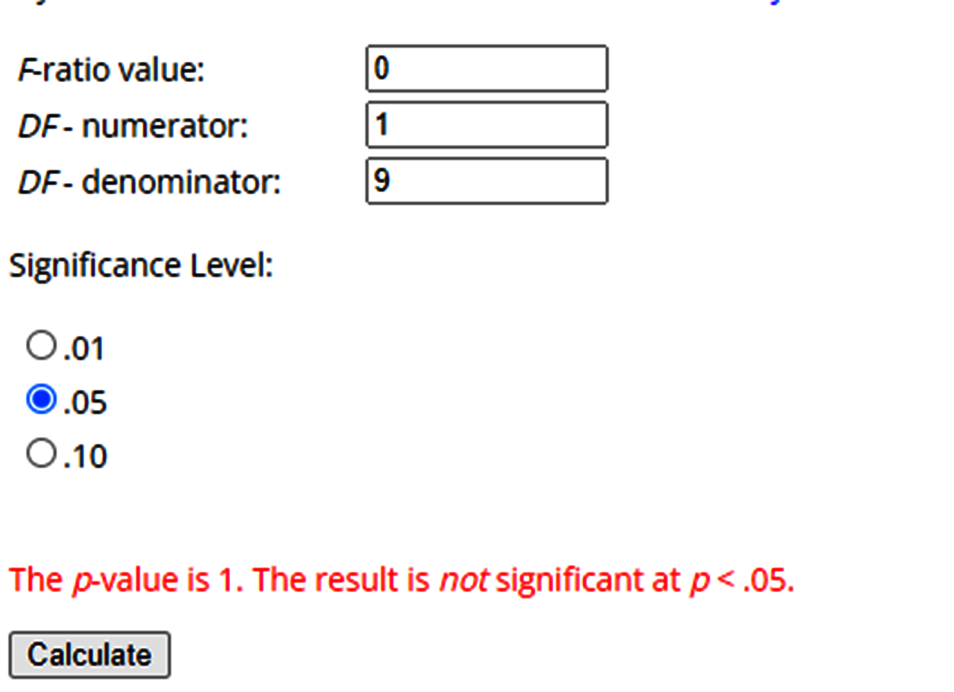
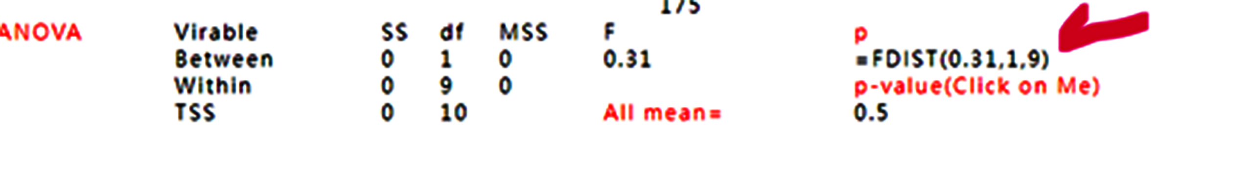
4.ANOVA
If ANOVA is selected, and the results shown below are identical to the previous ANOVA in the previous section based on group 1 in the label of input data.
2.Summary Table
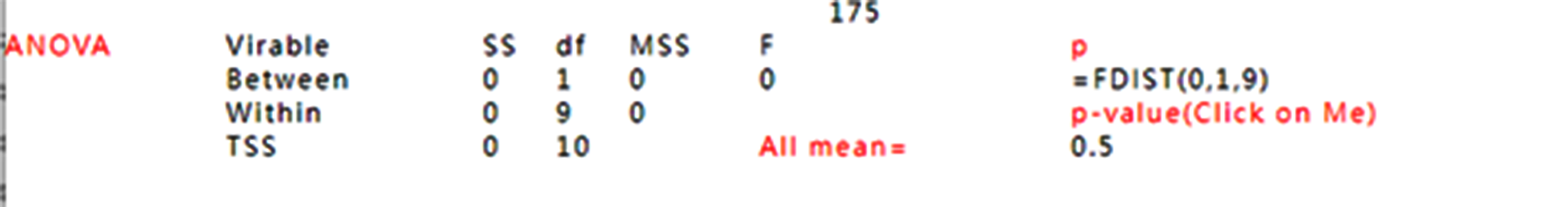
See the ANOVA table and the p-value for examining the difference in measures among groups
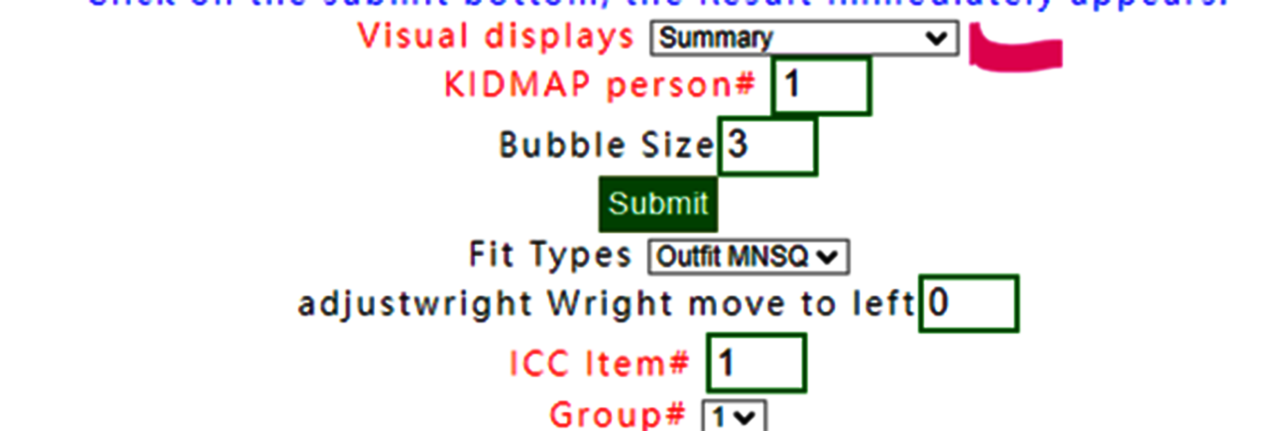
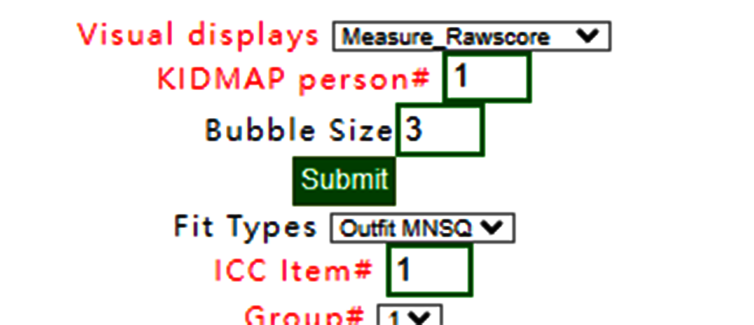
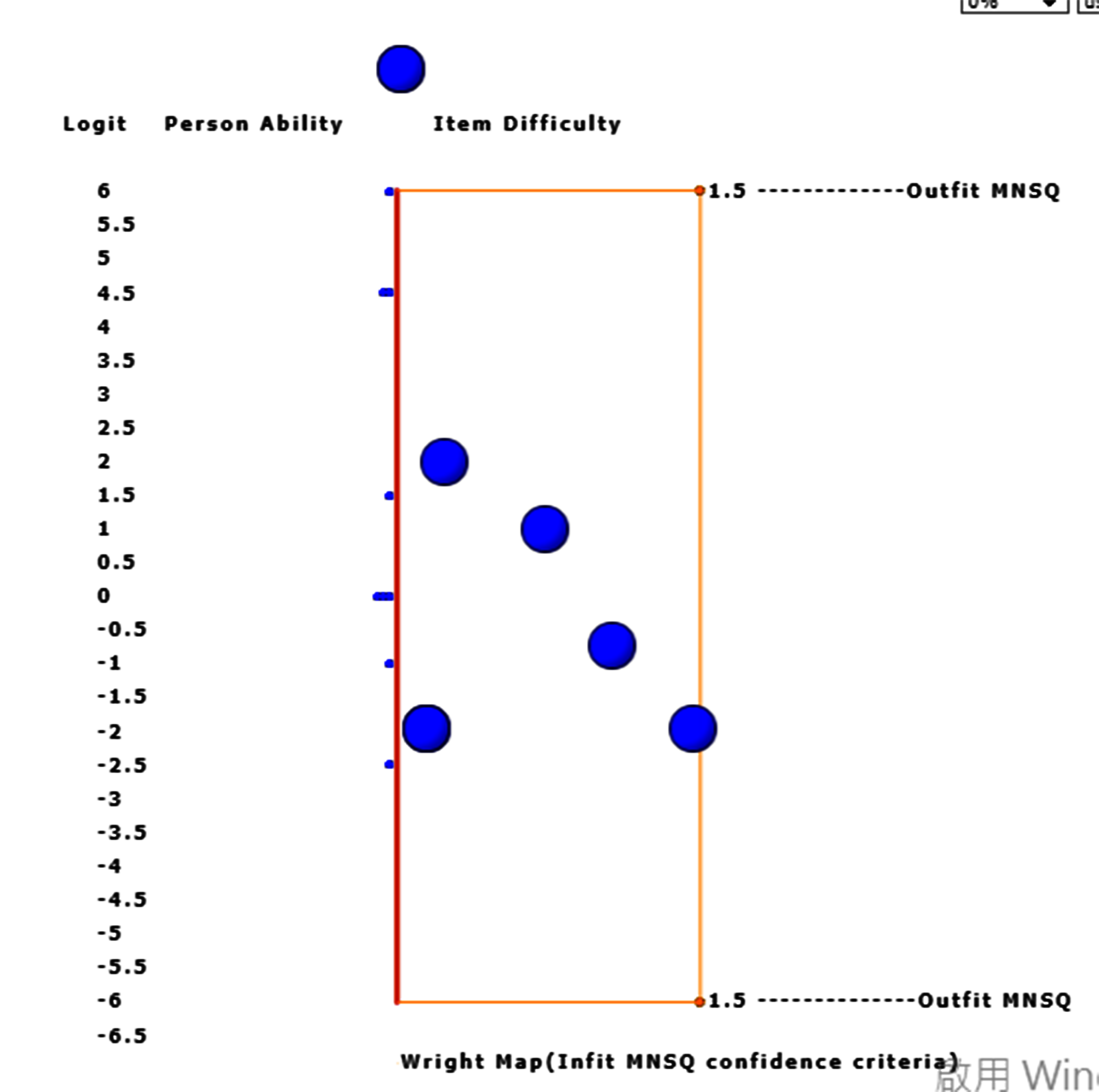
5.Wright Map
select Wright Map.
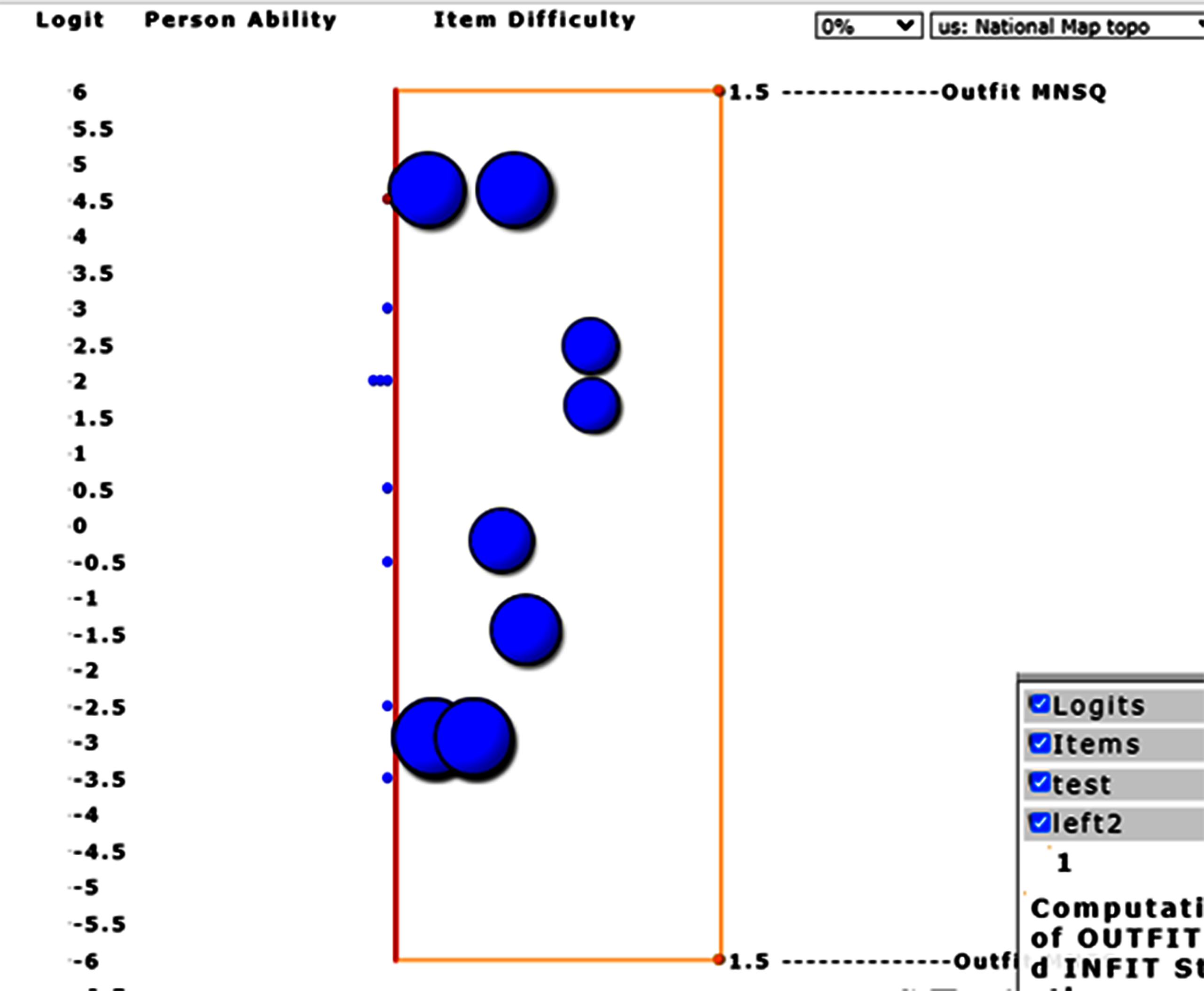
ToTodisplay Wright Map.
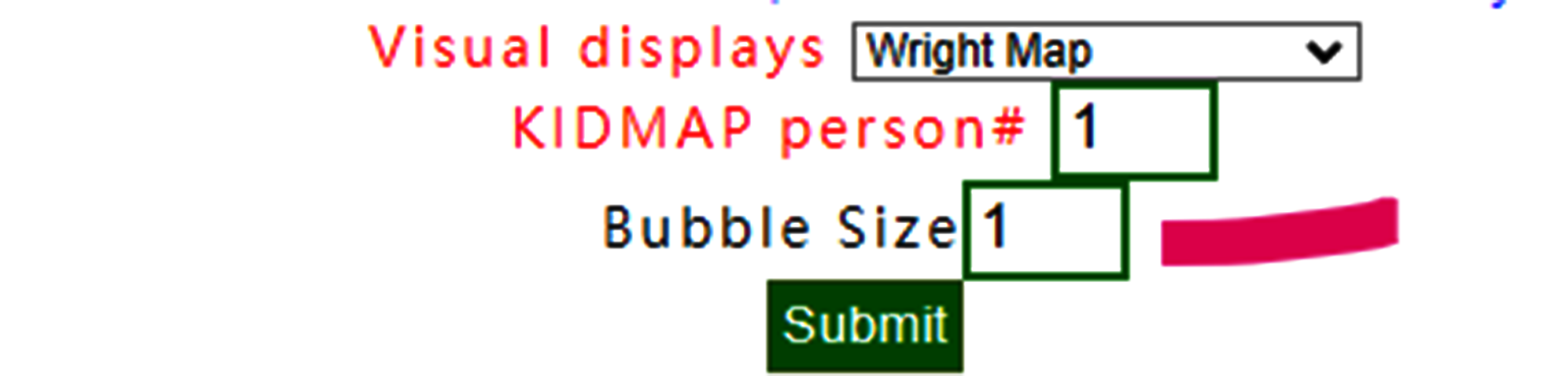
To adjust bubble size to 1
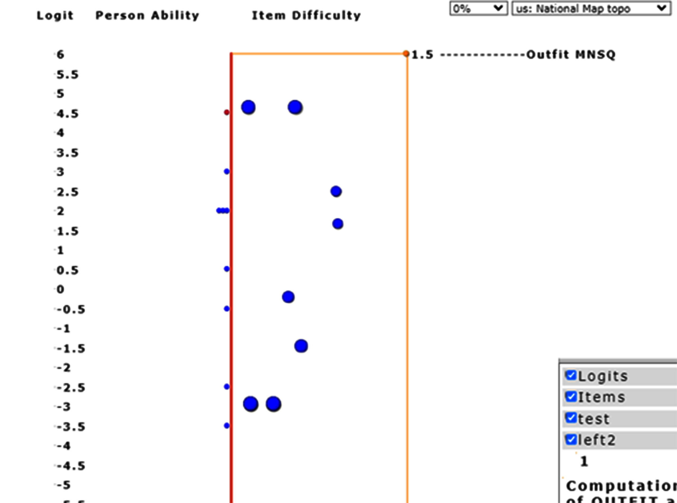
Bubbles are adjusted to an appropriate layout.
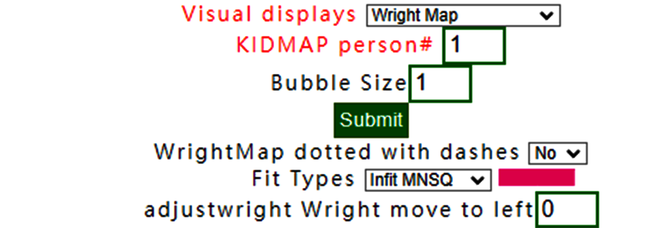
To adjust the fit statistics with infit
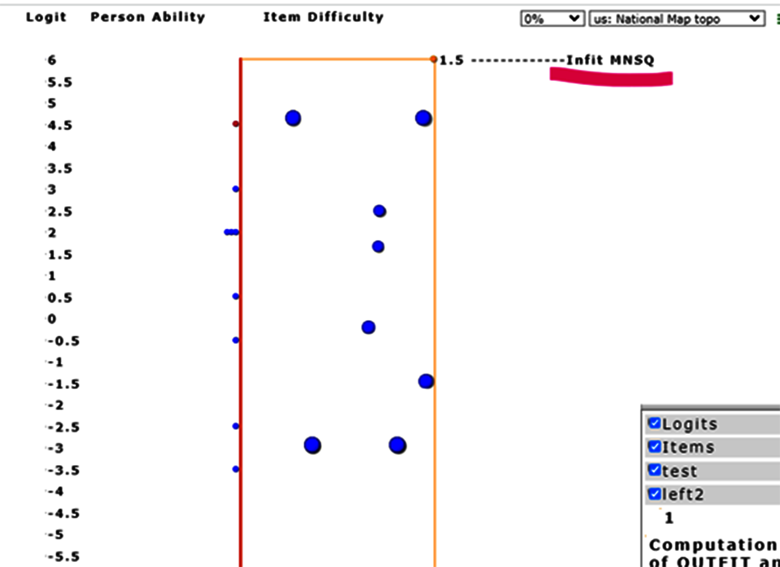
Item infit MNSQs are displayed, different from those with Outfit MNSQ in the previous example.
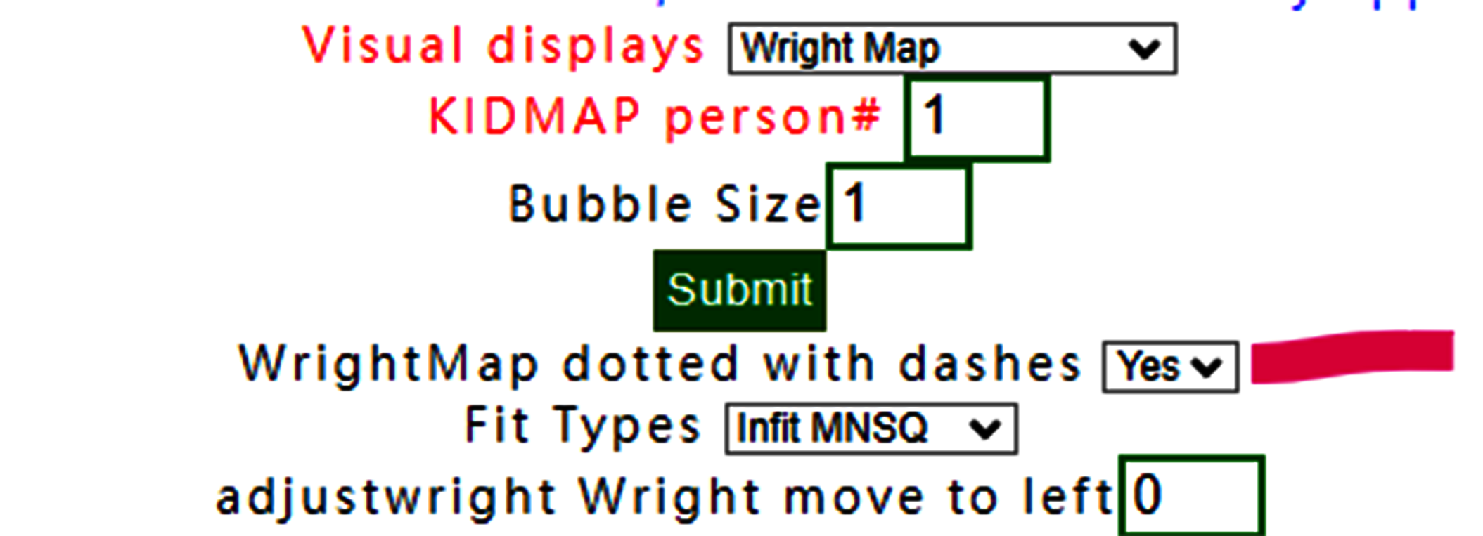
If dash is selected.
the results are identical due to no step difficulties in the dichotomous scale as shown below:.
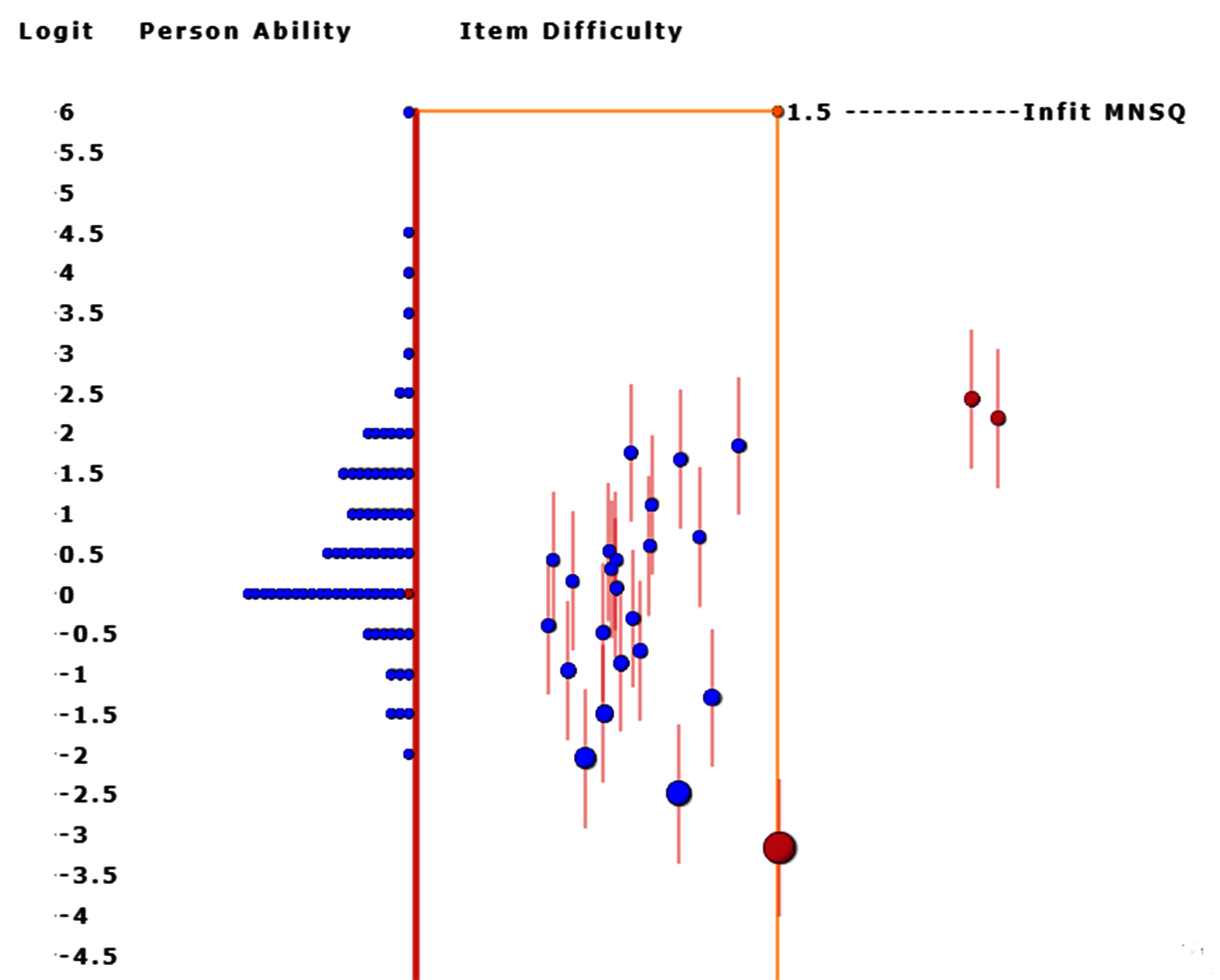
Otherwise, dashes are shown for RSM; see below.
6.Wright Map(Groups)
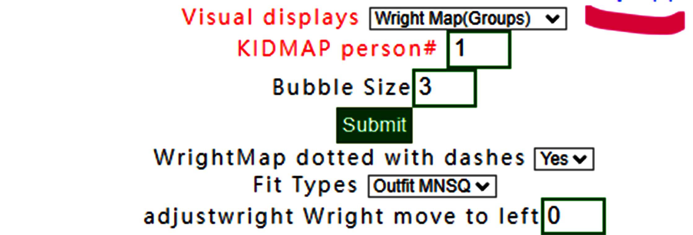
Wright Map with groups selected
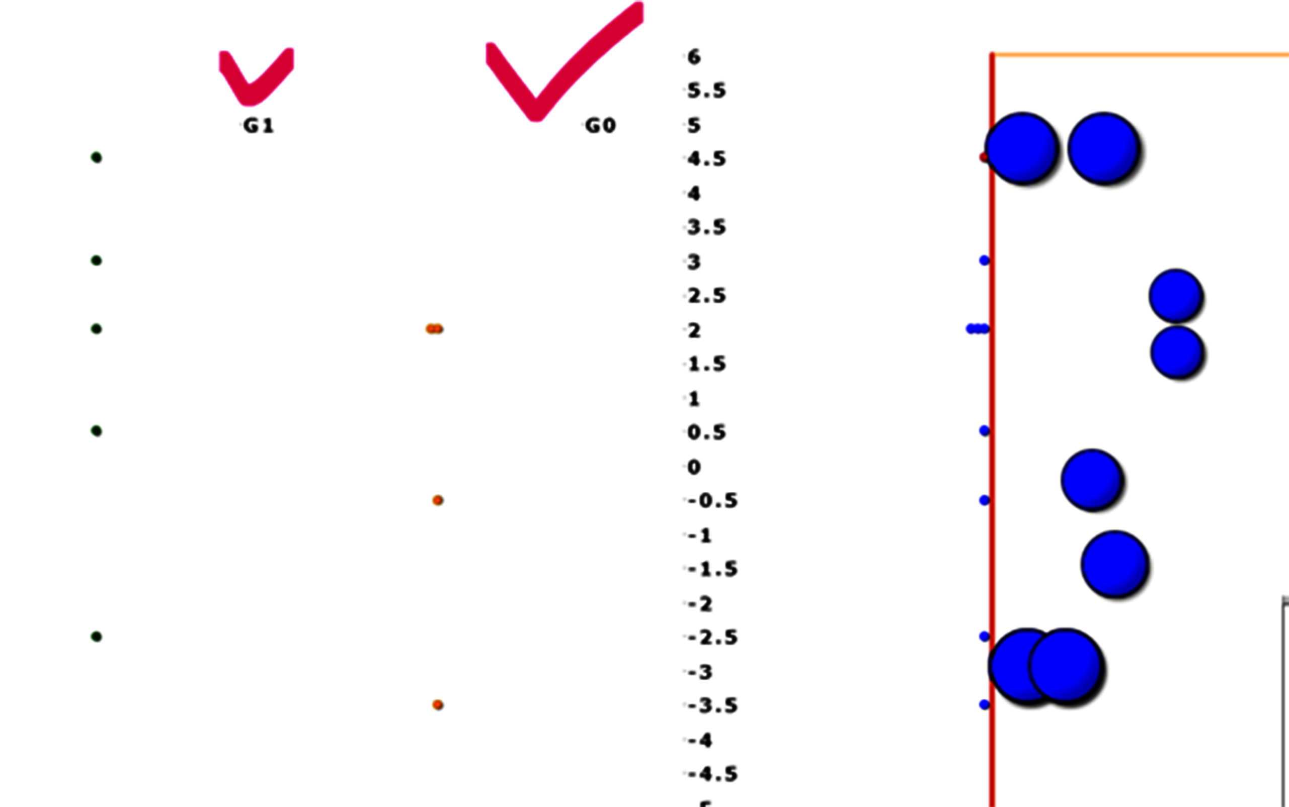
More distributions in groups are displayed on the left-hand side.
Note. the summation of numbers in groups are identical to the total counts on the right-hand side.
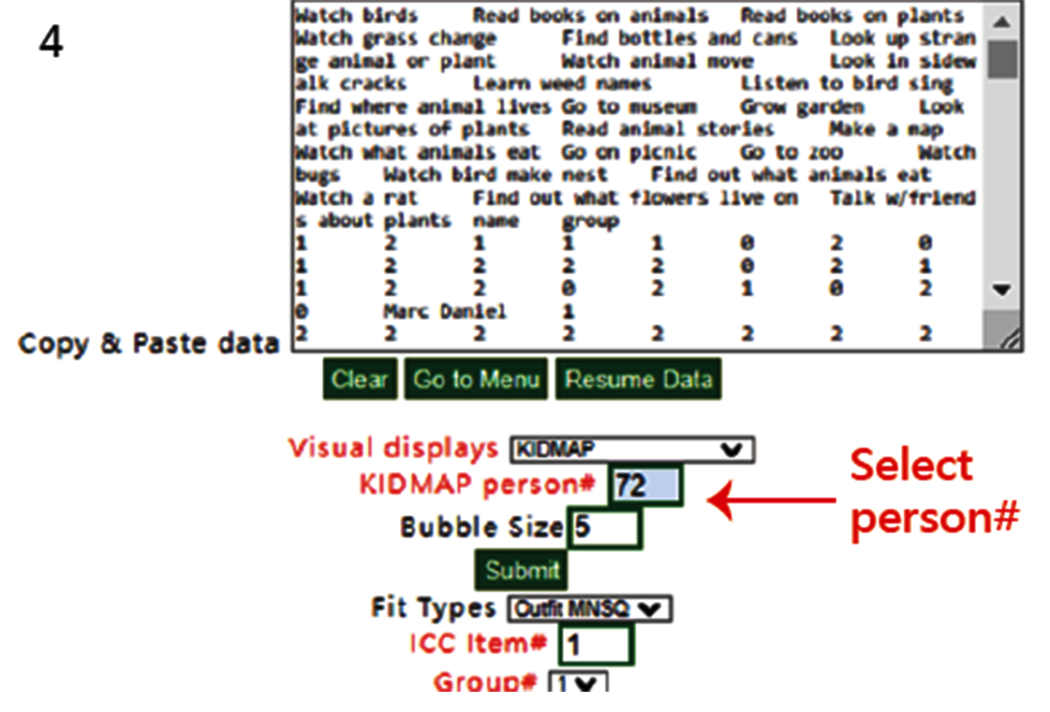
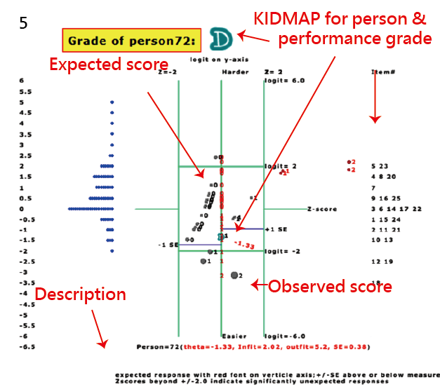
7.KIDMAP
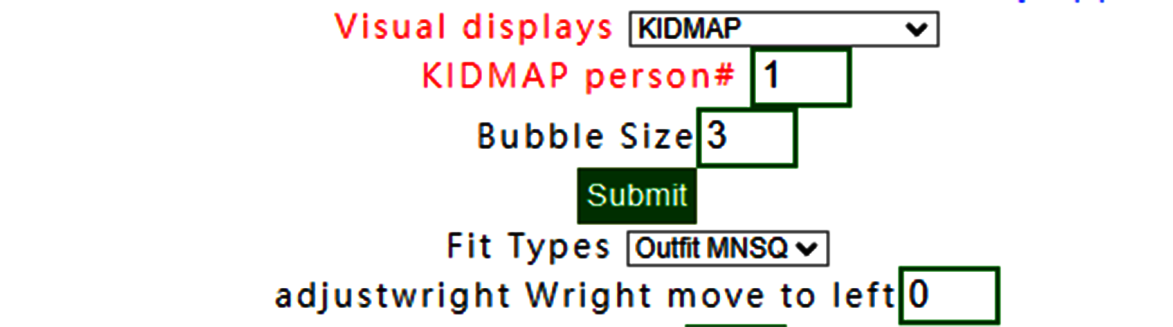
To select person number.
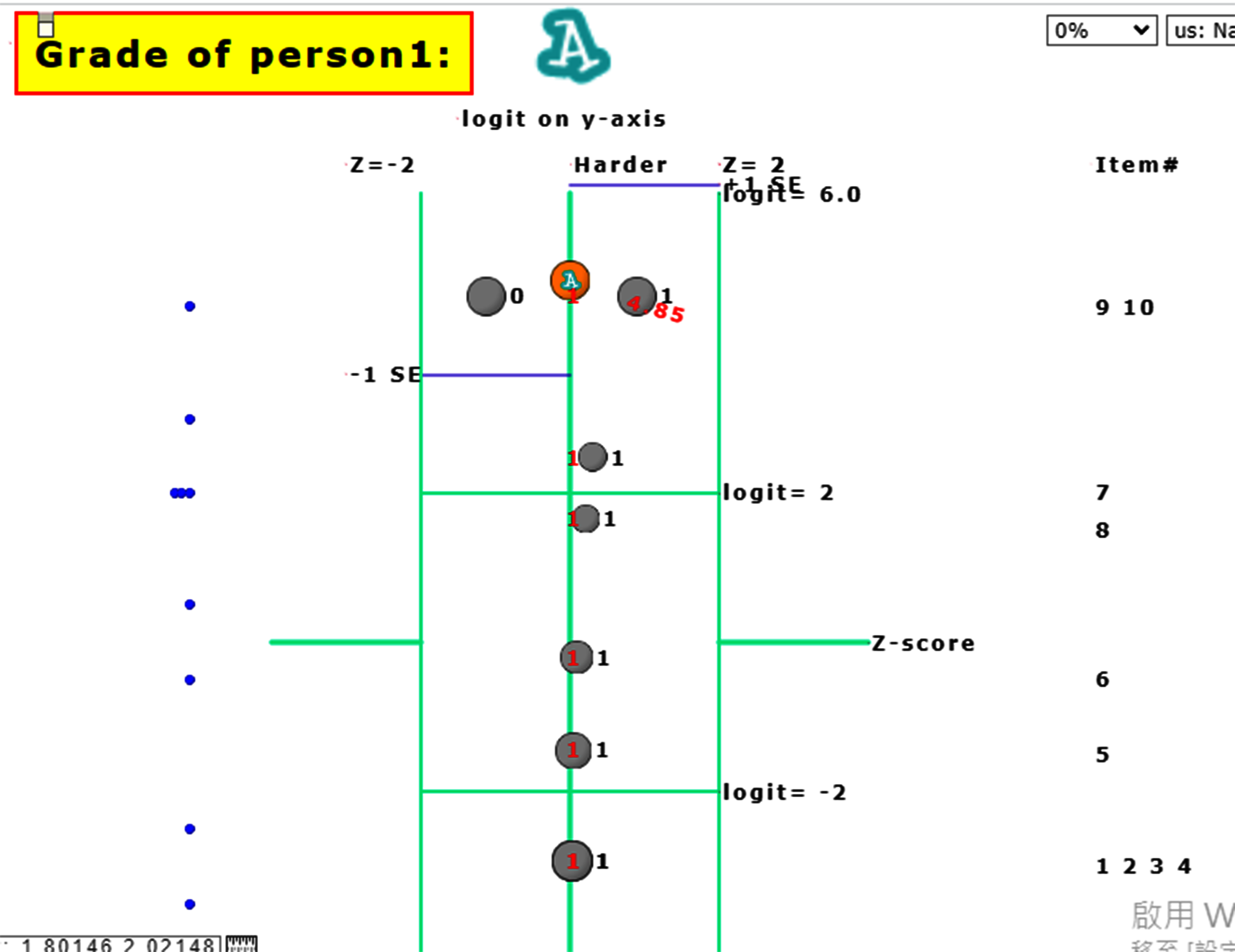
The one selected appears with a KIDMAP.
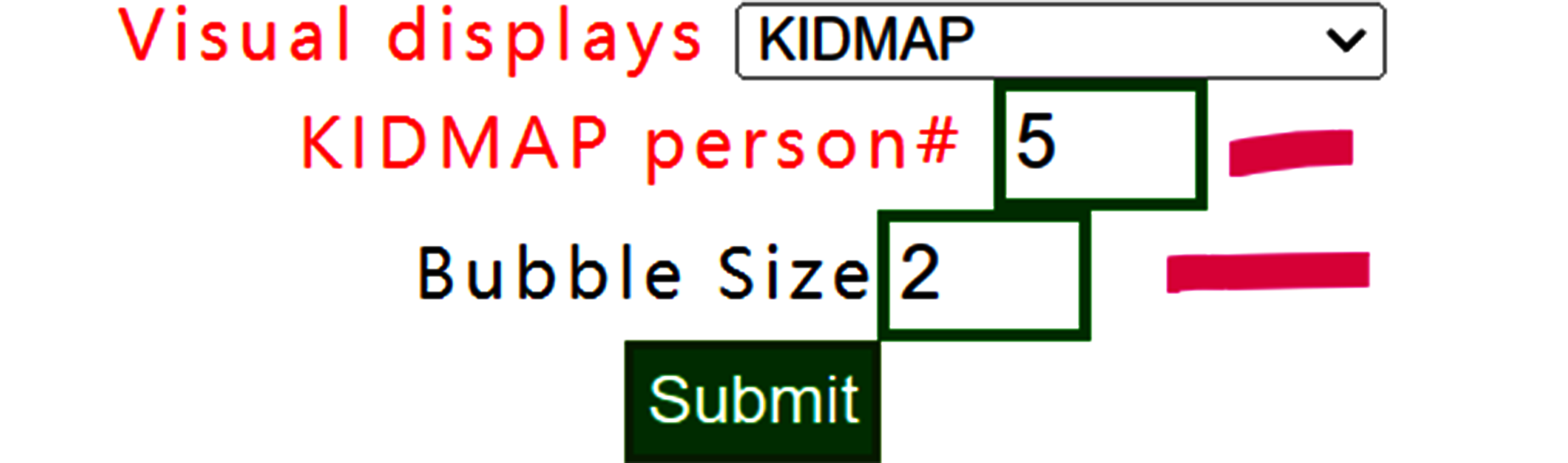
Another person is selected
Based on the person measure and fit statistics
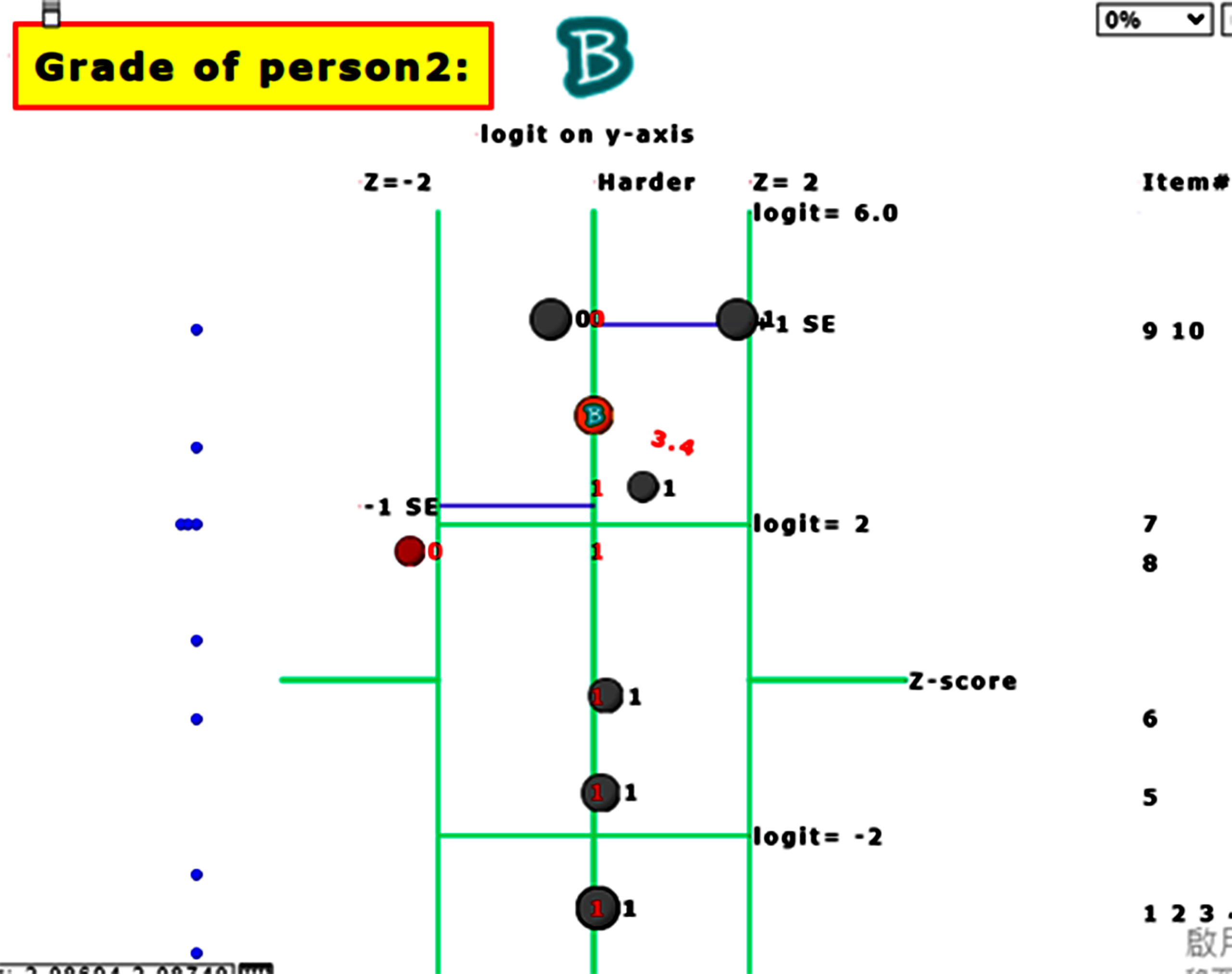
The one with one item unexpected is found using KIDMAP
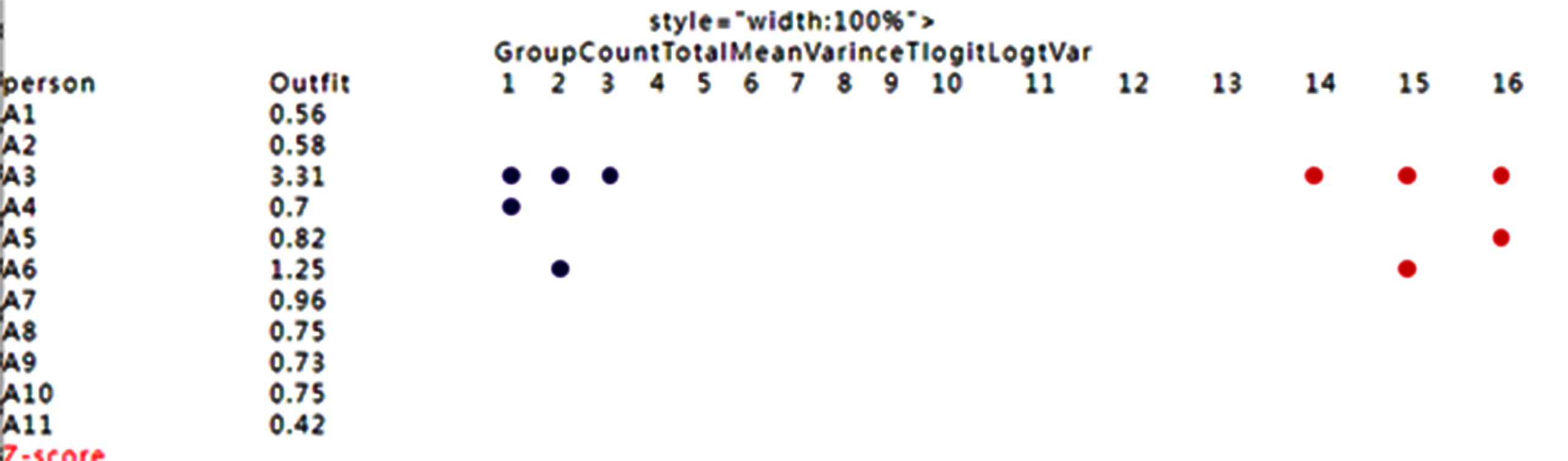
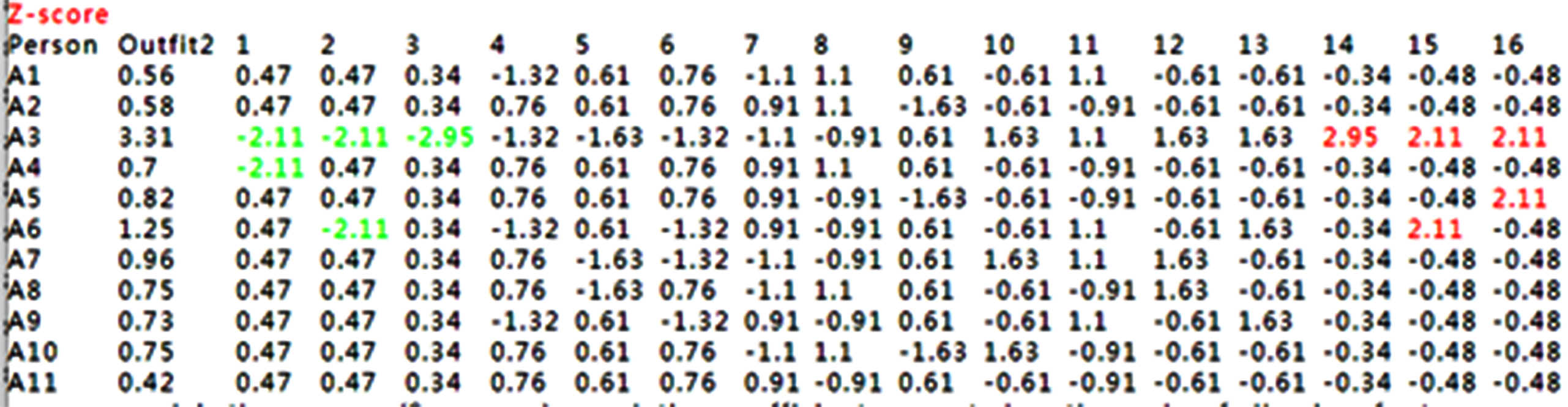
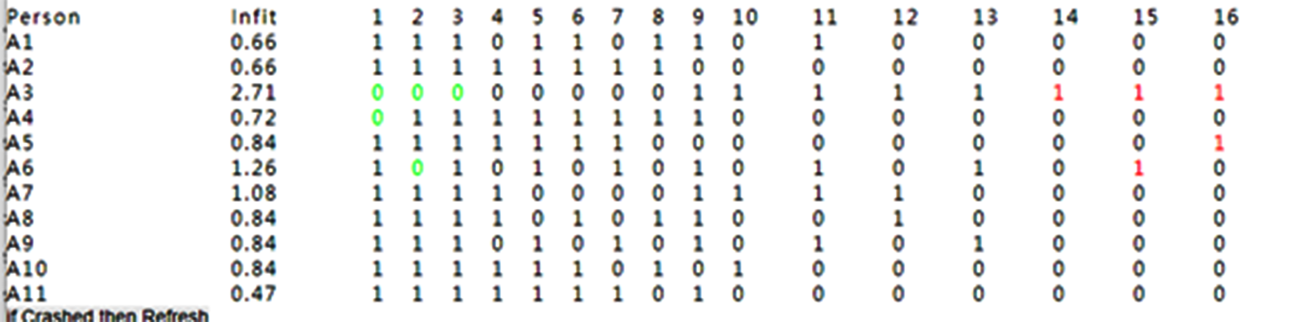
For person 2, we can see that item 8 in red bubble is unexpected(Zscore <-2.0) due to the easy item with incorrectness at the left-bottom side.
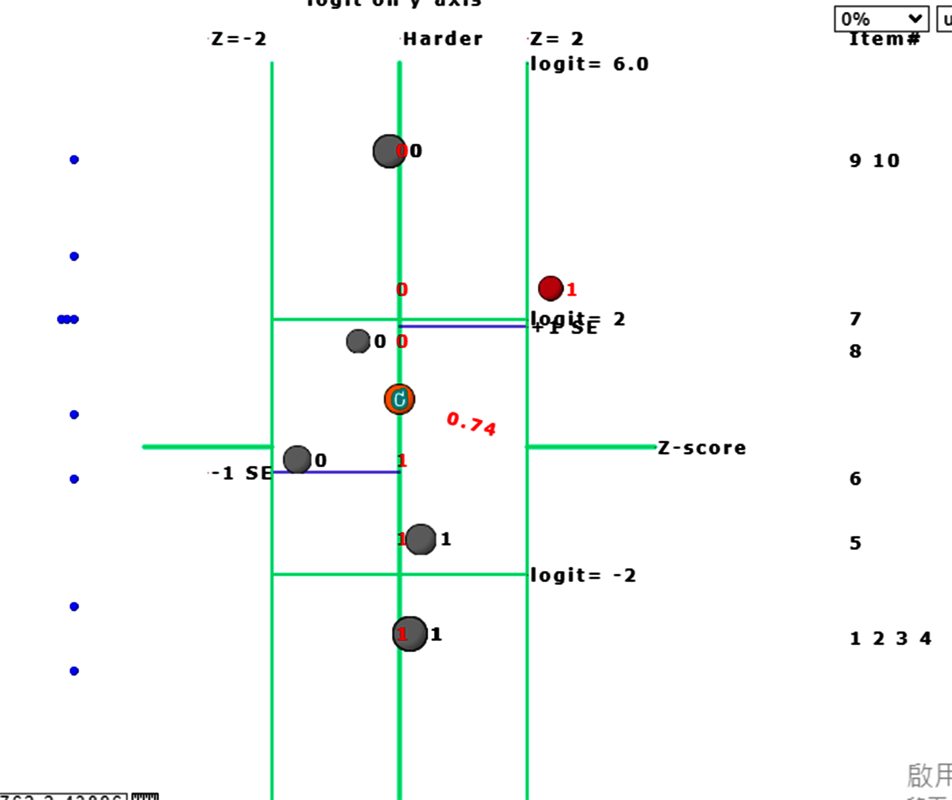
Another one with one item unexpected is found using KIDMAP.
For person 6, we can see that item 7 in red is harder but correct in the right-top side(Zscore>2.0)
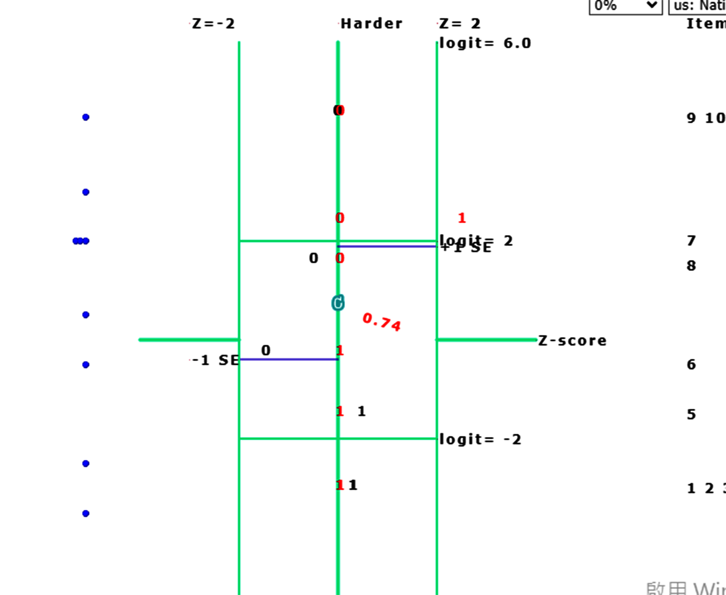
If bubbles were selected with smaller size, the KIDMAP can be clear with expected and observed responses across items along with difficulties from top to bottom.
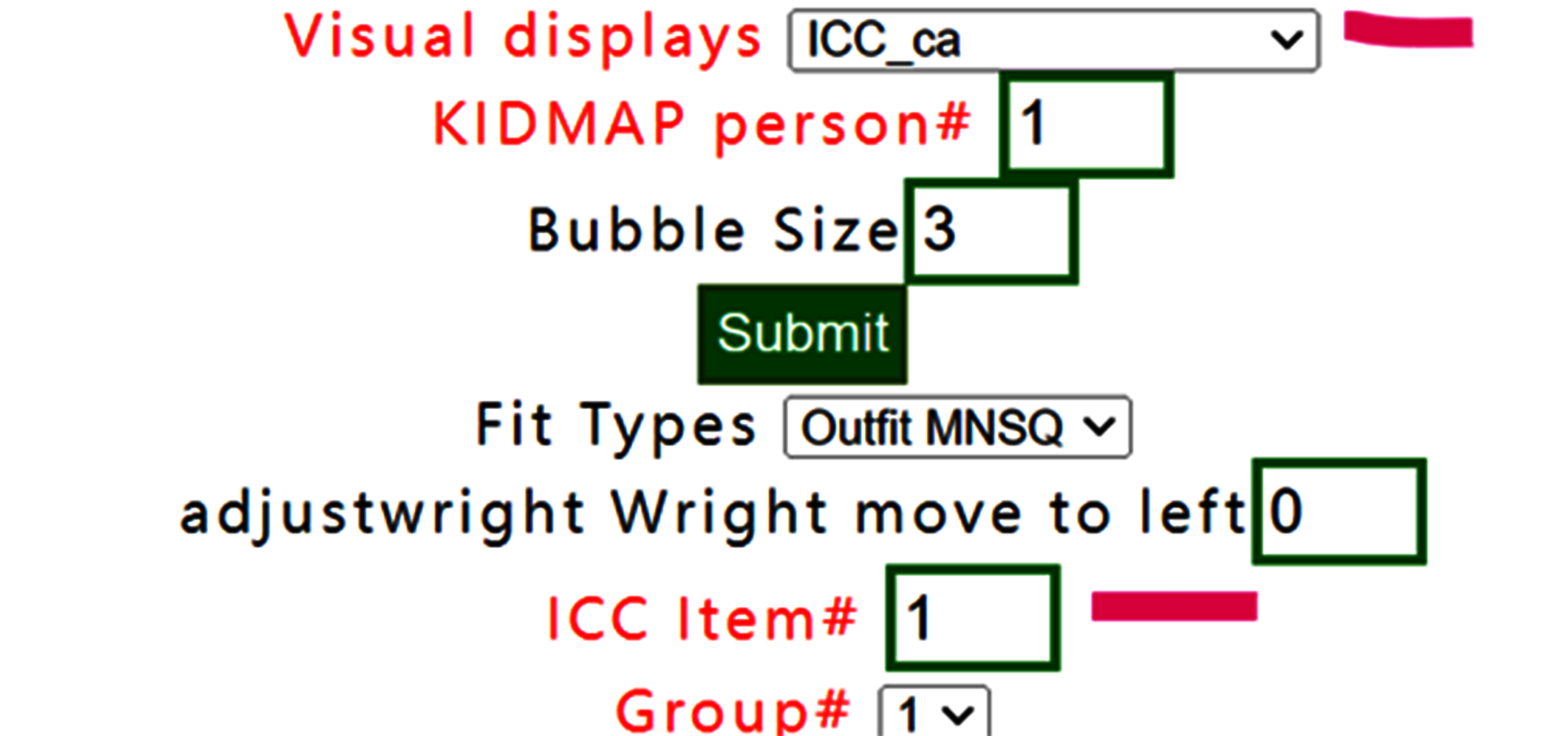
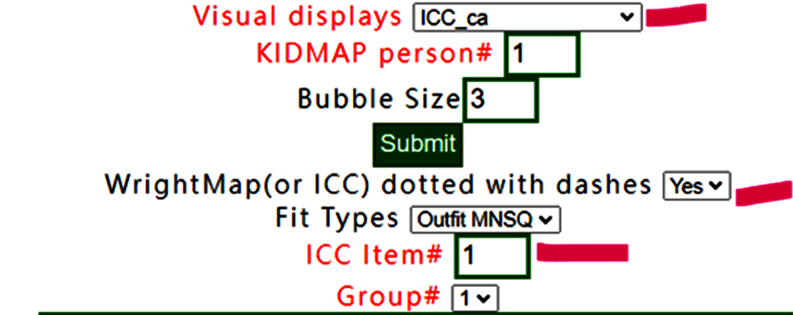
8.ICC_cat
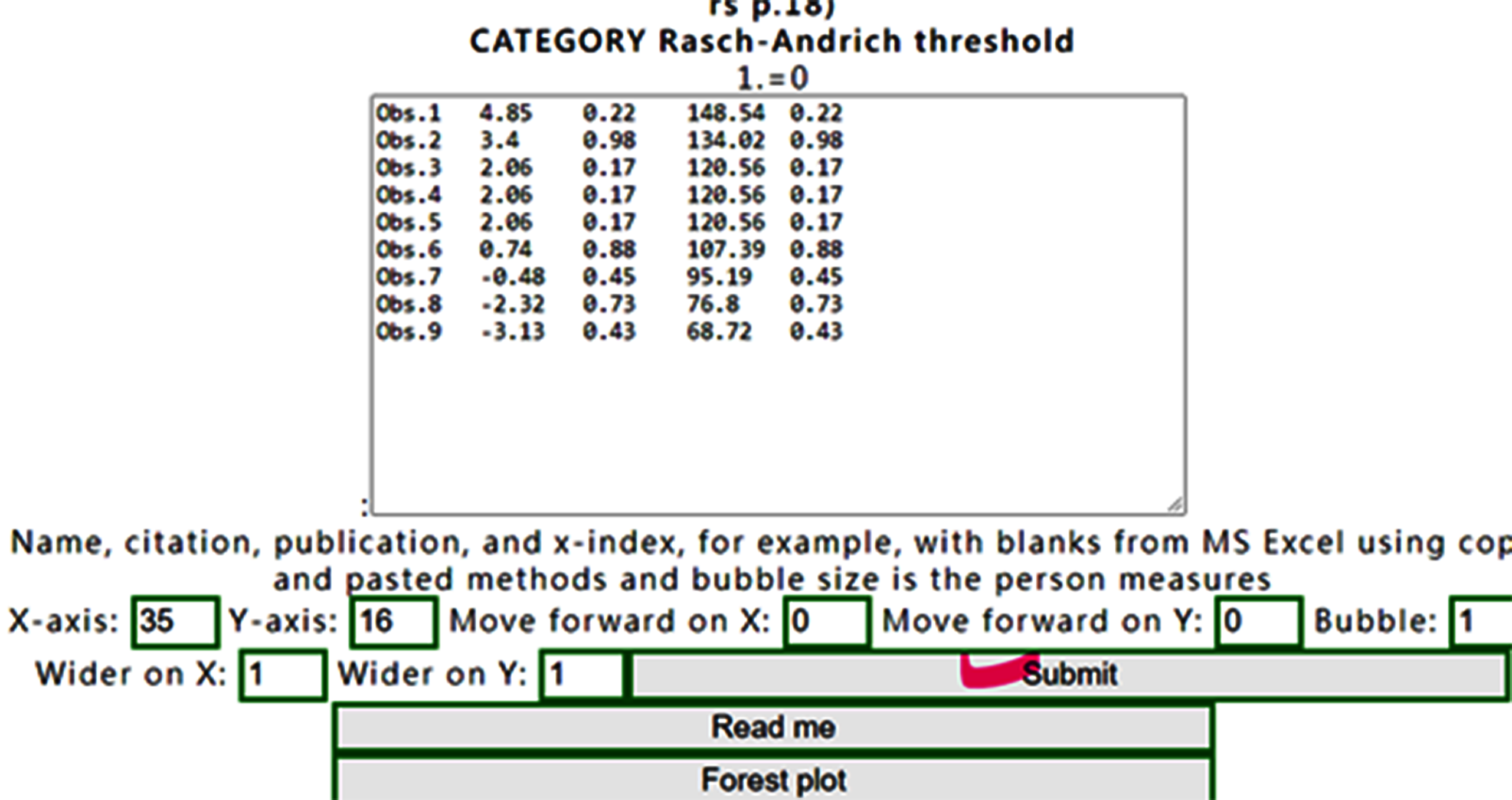
The CATEGORY PROBABILITIES: MODES - Andrich thresholds at intersections with ICC shows item# 1 for all persons below:
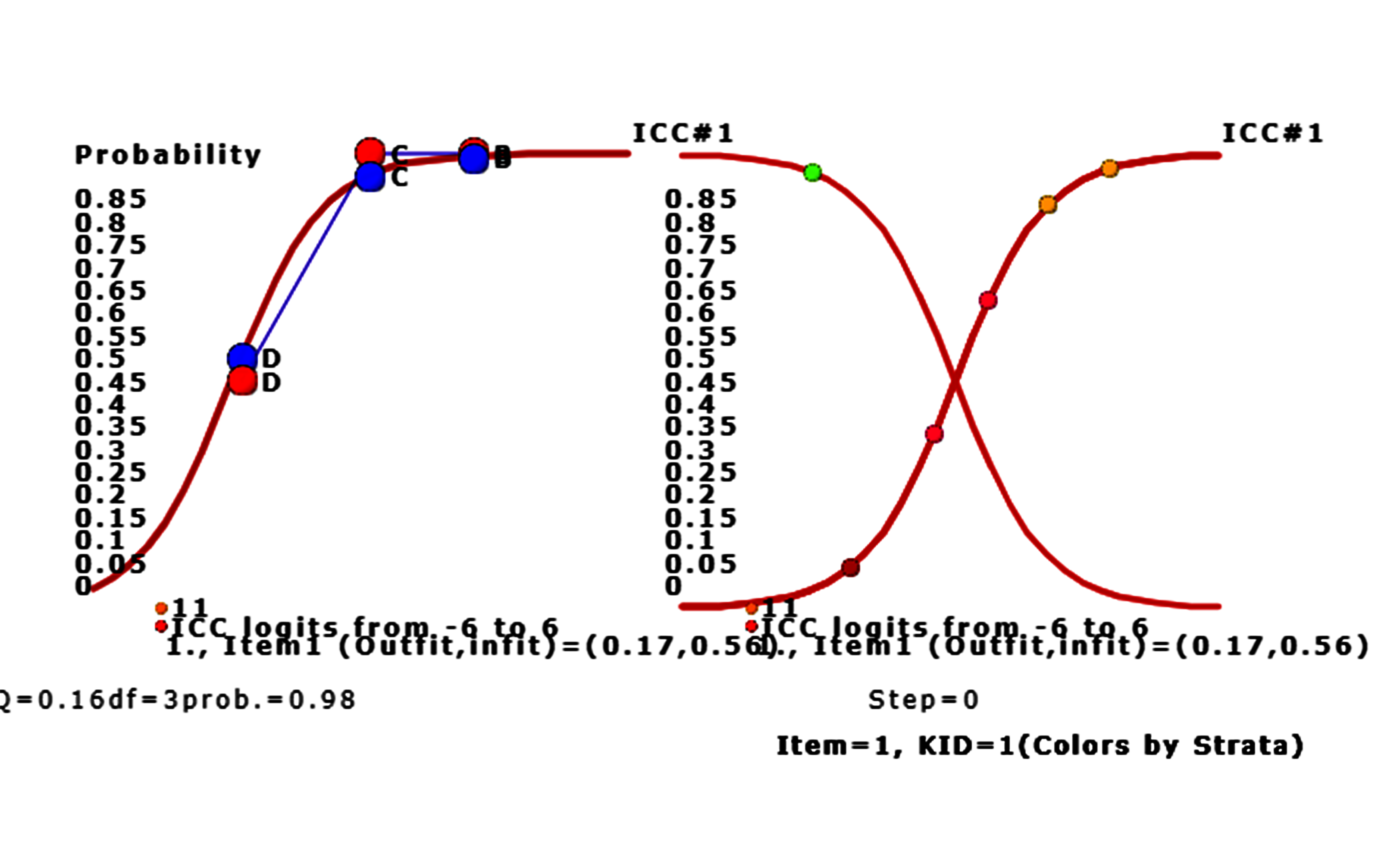
We can see that only person 9 answers tem 1 incorrectly. Other persons answer item 1 with correctness on the success ogive cure for left-bottom to right-top corner.
Persons with higher ability are on the right-hand side. The bubble denoted by the vertical probability corresponds to the person ability.
Moving to the left on Google Maps, the ICC of item 1 is shown above. The red bubbles denote the observed responses by persons and the blue ones represent the expected responses by persons. The ChSQ statistics shown below, similar to the overall fit selected in the menu at the beginning.
Bubbles are colored by groups. We can see that only person 9 answers item 1 incorrectly. Other persons answer the item 1 with correctness on the success ogive cure for left-bottom to right-top corner.
Persons with higher ability are on the right-hand side. The bubble denoted by the vertical probability corresponds to the person ability.
To add lines linked to observed bubbles in ICC
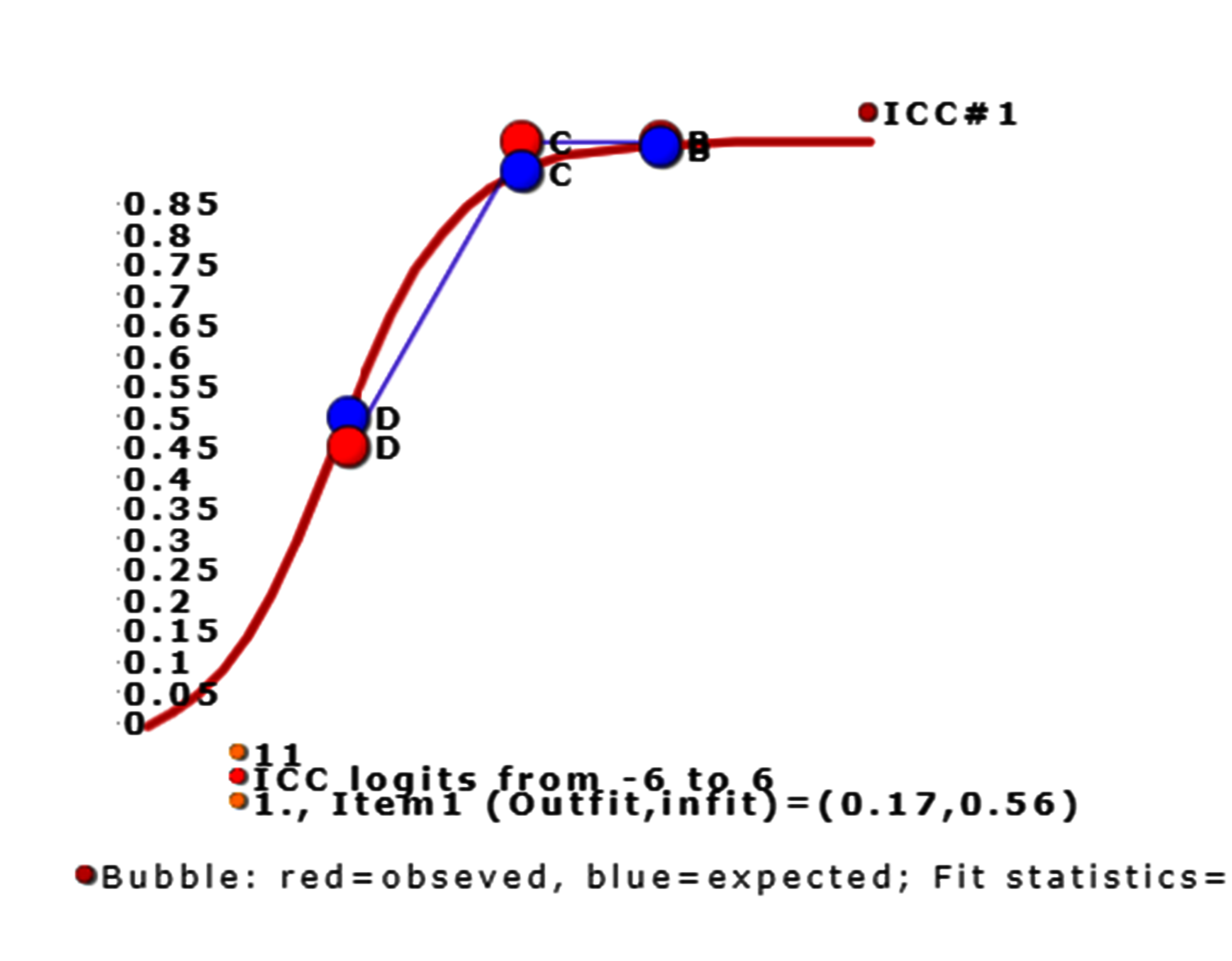
The lines have been linked for observed responses of groups.
Why the ICC has six persons, but nine person in the dataset, which is the reason for the three persons have identical measures and make the bubble overlaid together.
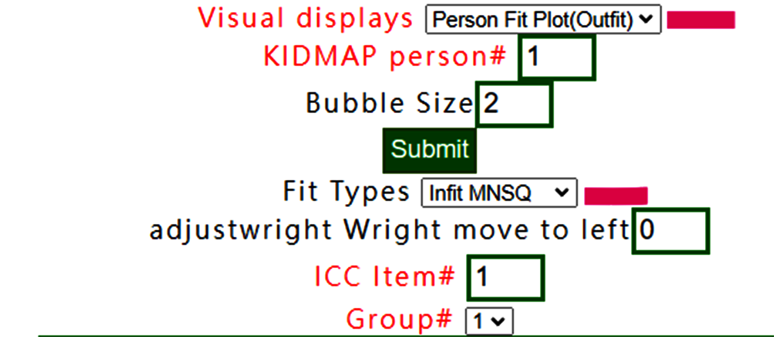
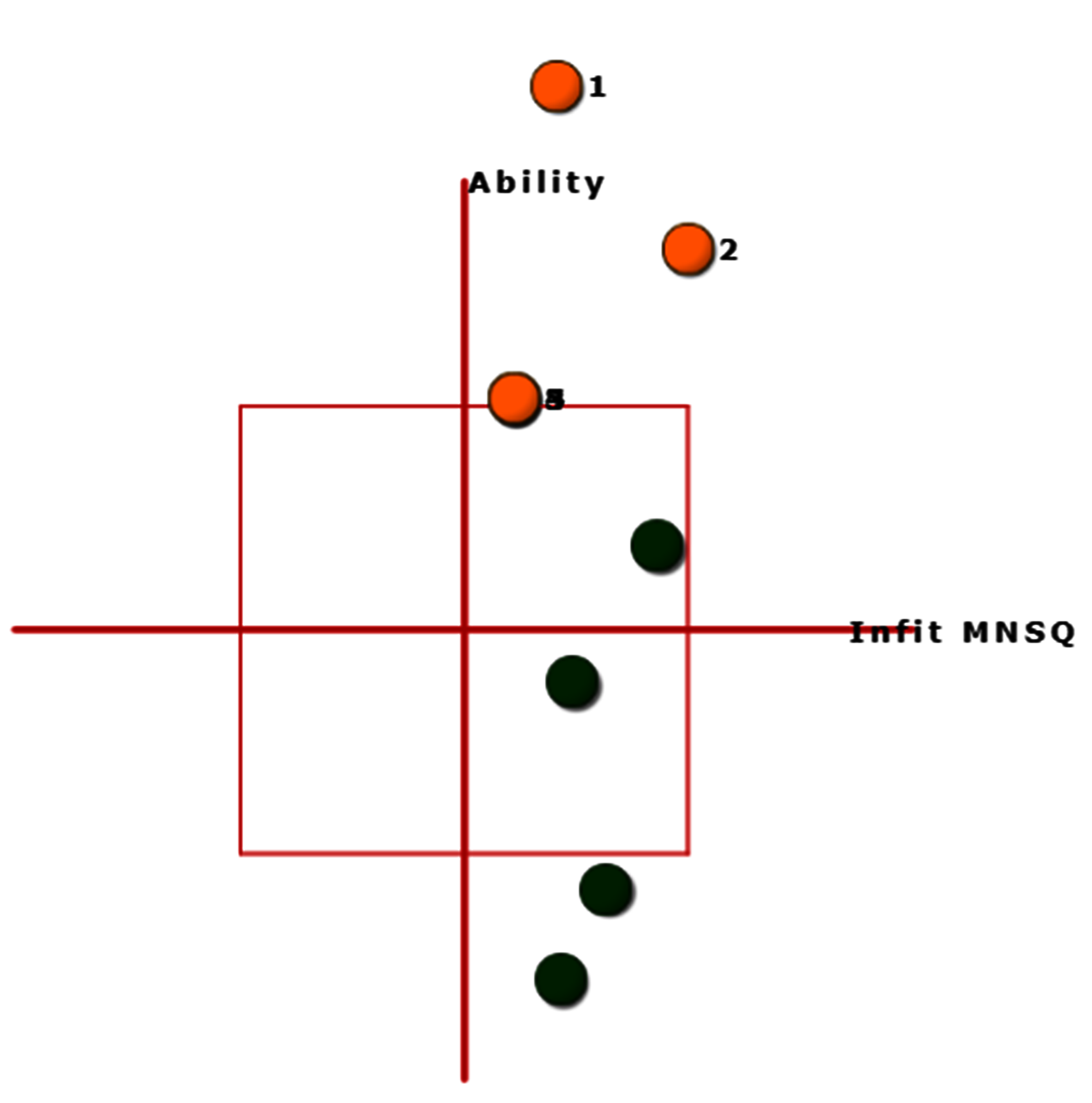
9.Person fit plot(Outfit)
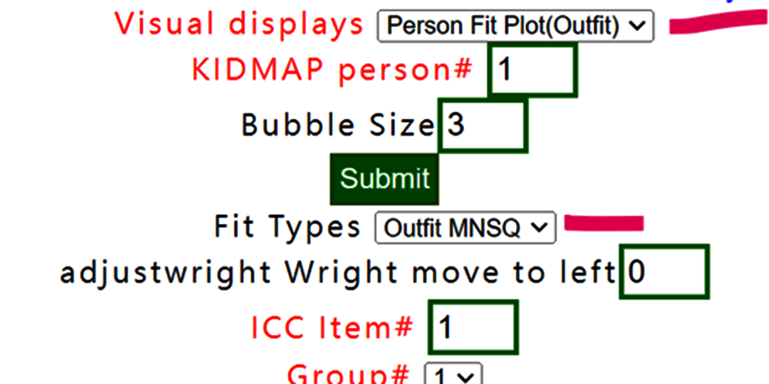
Select person fit plot with outfit MNSQ,
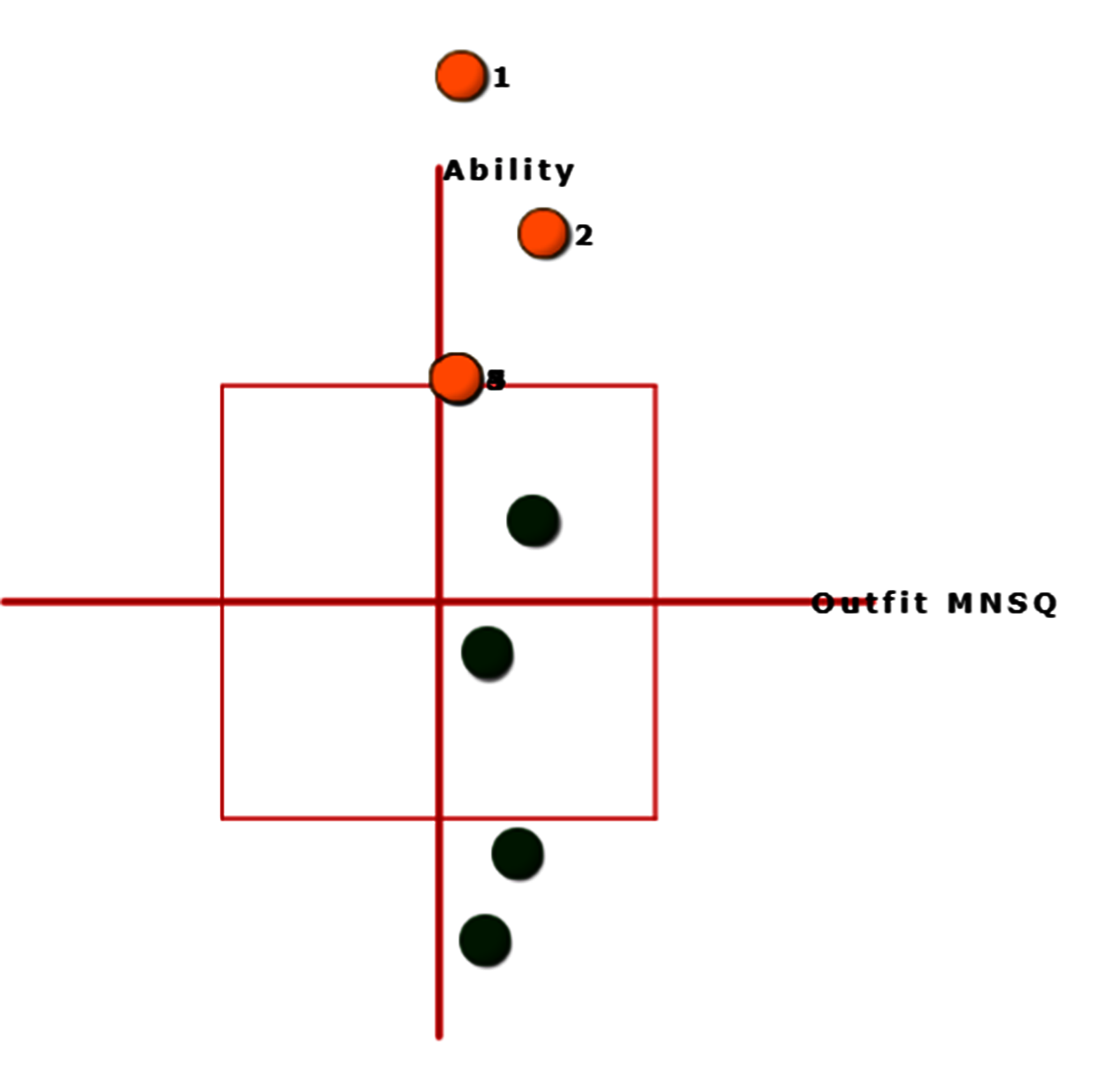
Outfit MNSQs are on the x-axis and person abilities are on the vertical y-axis. Bubbles are sized by person SE. In this case, we observed that all persons have outfit less than 2.0.
10.Person fit plot(Infit)
If Infit MNSQ is selected, the person fit plot is shown below:
Bubbles are sized by person SE and shown with infit MNSQ.
11.Measure/Outfit
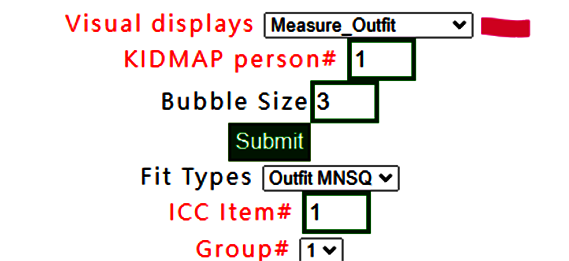
Measure Outfit is selected.
The buffered form is generated. After confirming it, the plot is shown as below:
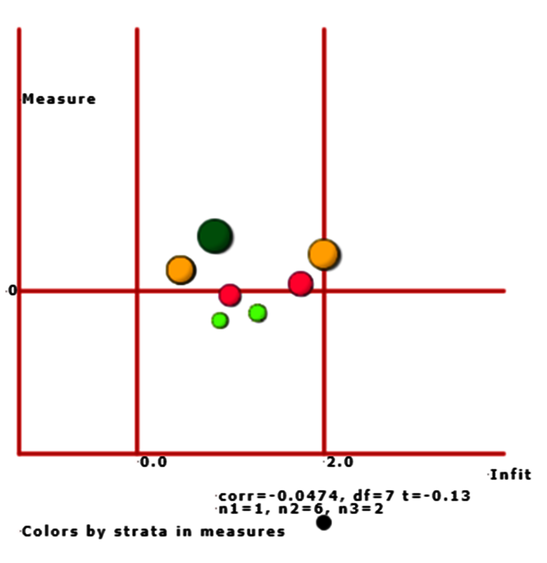
As the scatter plot shows the relationship between Outfit MNMS and person measure, three parts with colors are shown based on person strata.
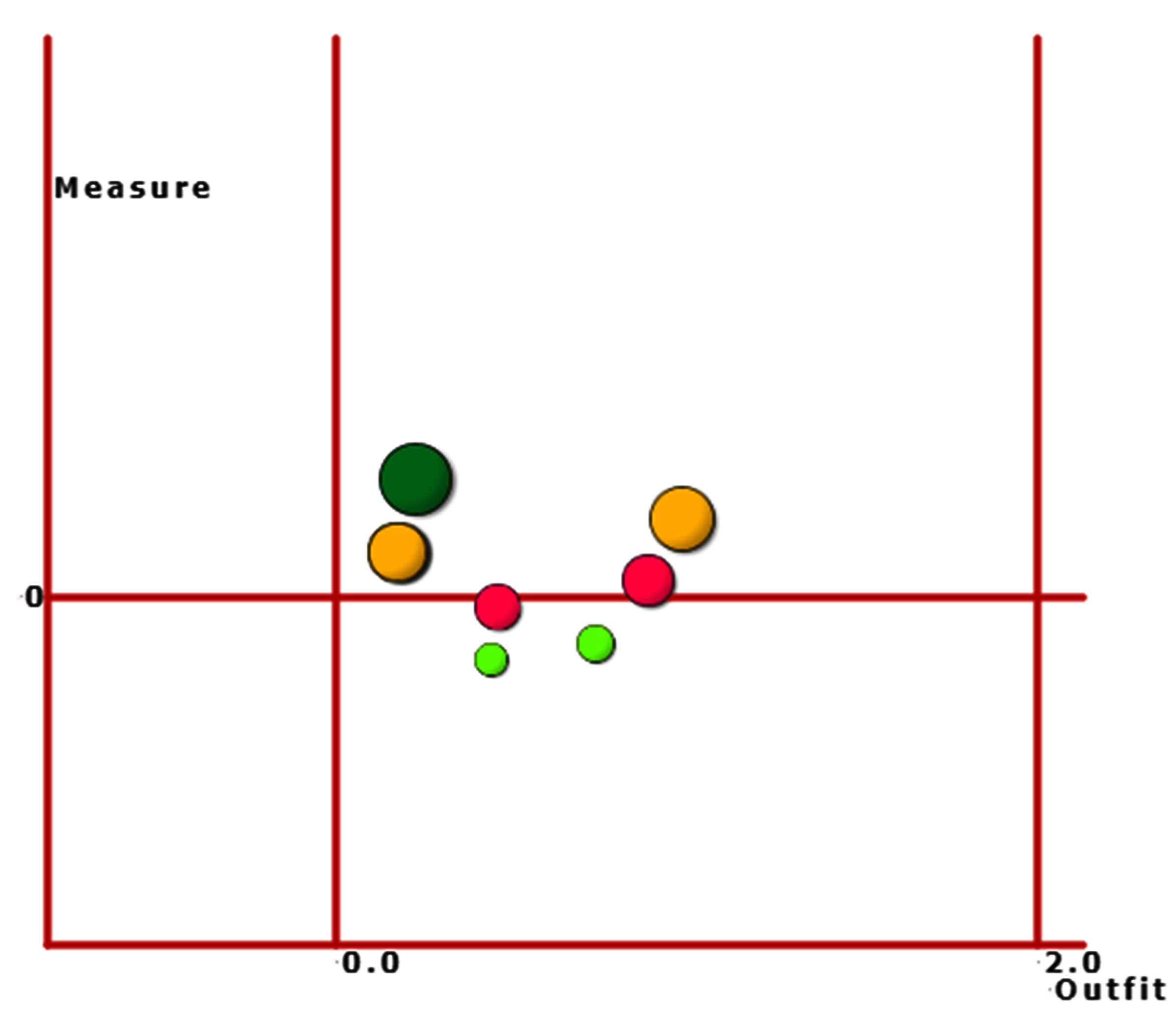
12.Measure/Infit
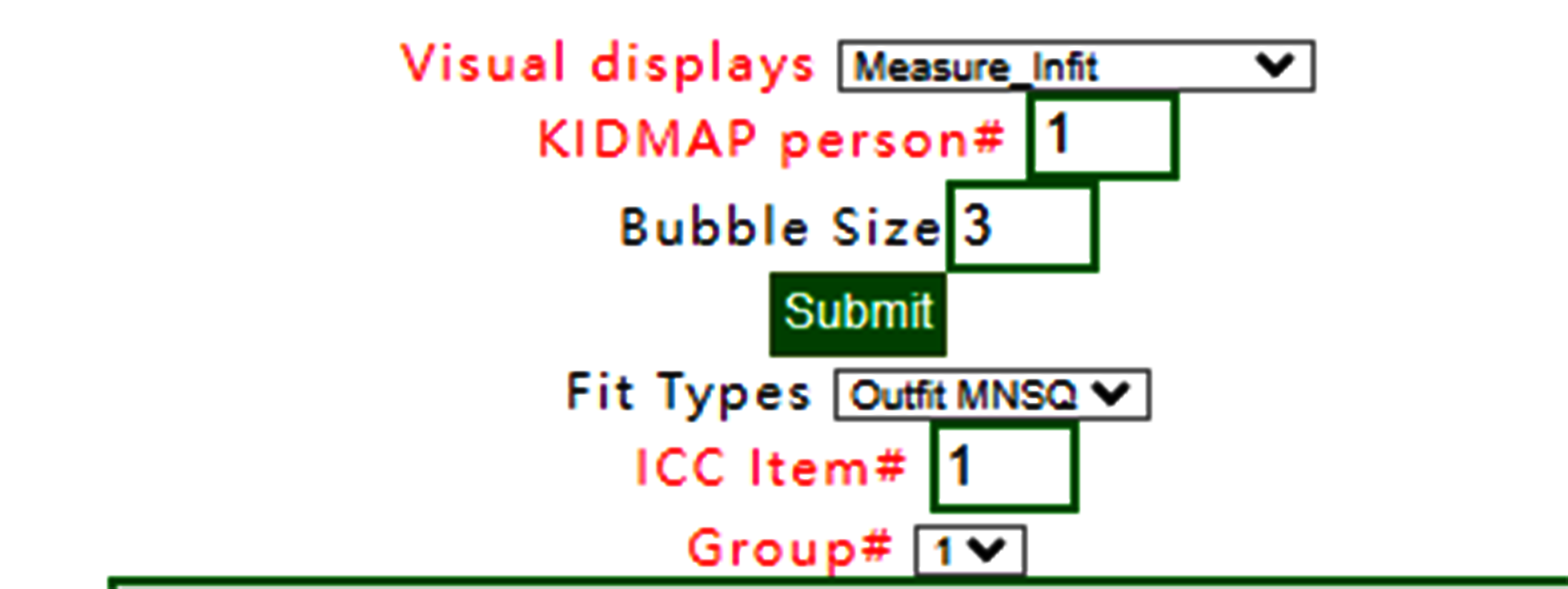
Measure Infit is selected.
The buffered form is generated. After confirming it, the plot is shown as below:
As the scatter plot shows the relationship between Infit MNMS and person measure, three parts with colors are shown based on person strata.
13.Rawscore/Measure
When Rawscore/measure plot is selected using Kano diagram, the confirmation is shown below:
Confirm it and show the Kano diagram below:
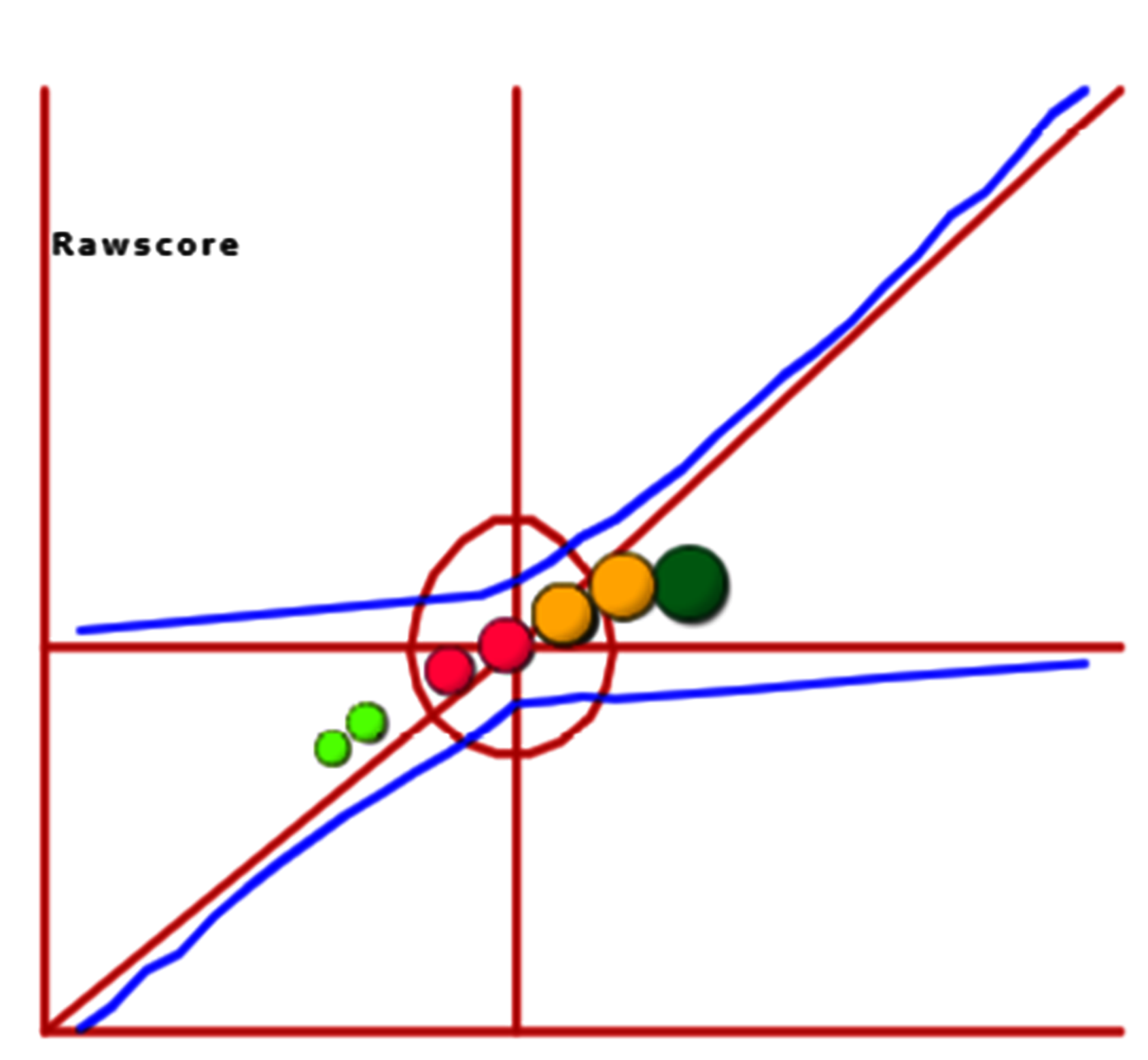
We can see that all person measures are along with raw scores on the one-dimensional part in the diagram.
The correlation coefficient is 0.9758 shown below the plot.
14.Simulation data
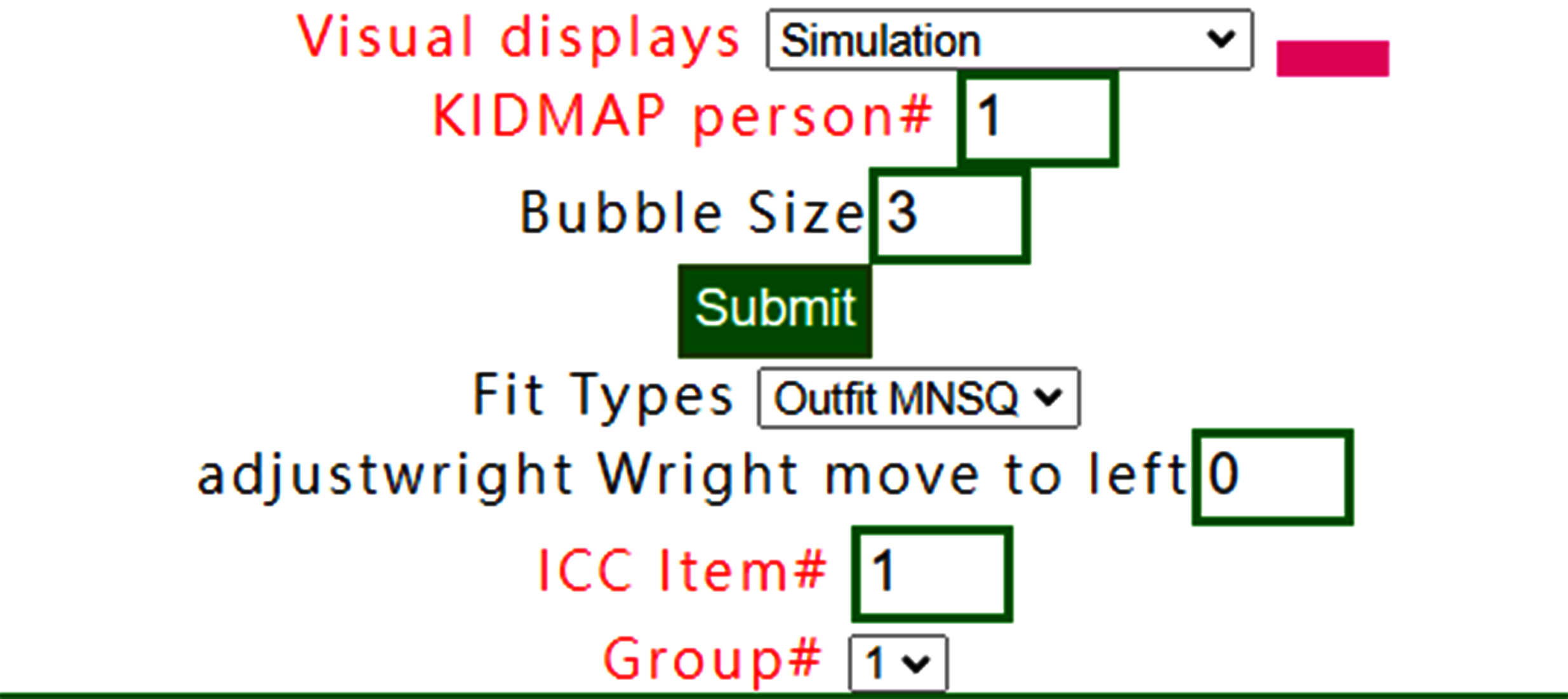
The simulation data can be generated based on the reference at https://www.rasch.org/rmt/rmt213a.htm
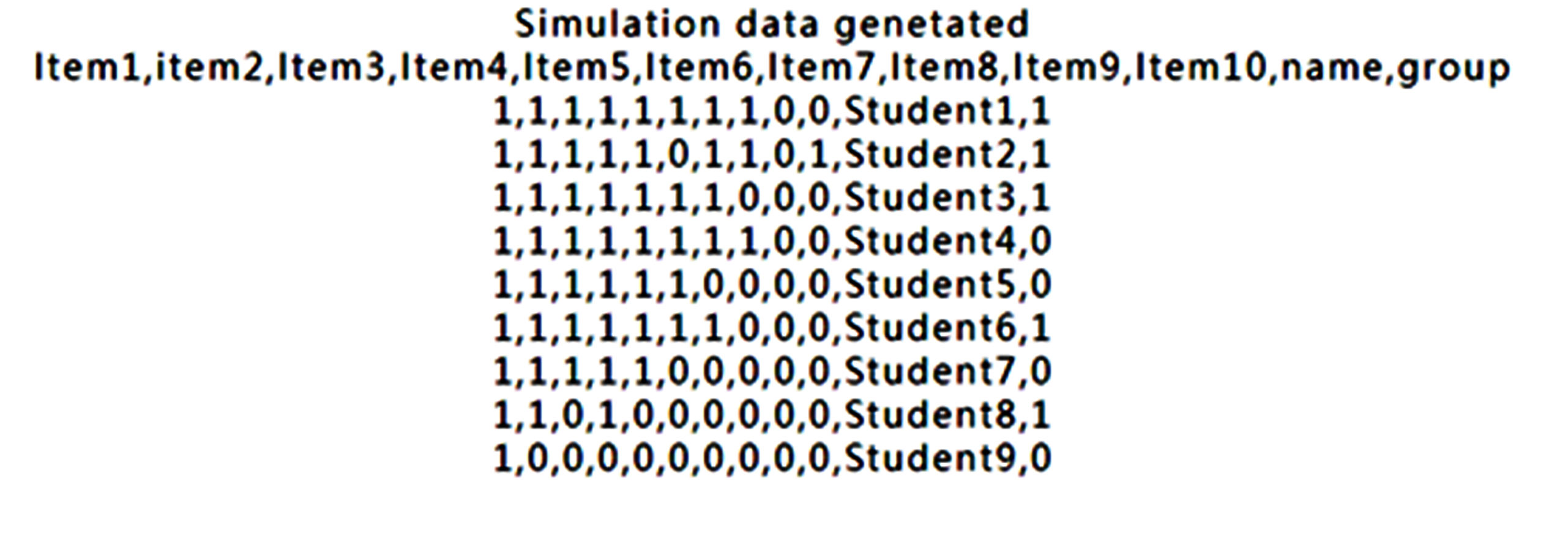
The result below the website is the simulation data. We copy those data onto RaschOnline.
We can see that all person measures are along with raw scores on the one-dimensional part in the diagram.
Like this one above. If the visual display with None is selected, the results show all items fit to Rasch model when observing all infit/outfit MNSQ smaller than those in the original dataset.
See how well items fitting to the Rasch model
That is because the data fit Rasch model fairly well.
However, the two with extreme measures have larger standard errors in measures using Wright Map to display.
When the bubble of interest is clicked, the detailed information about the item appears on Google Maps.
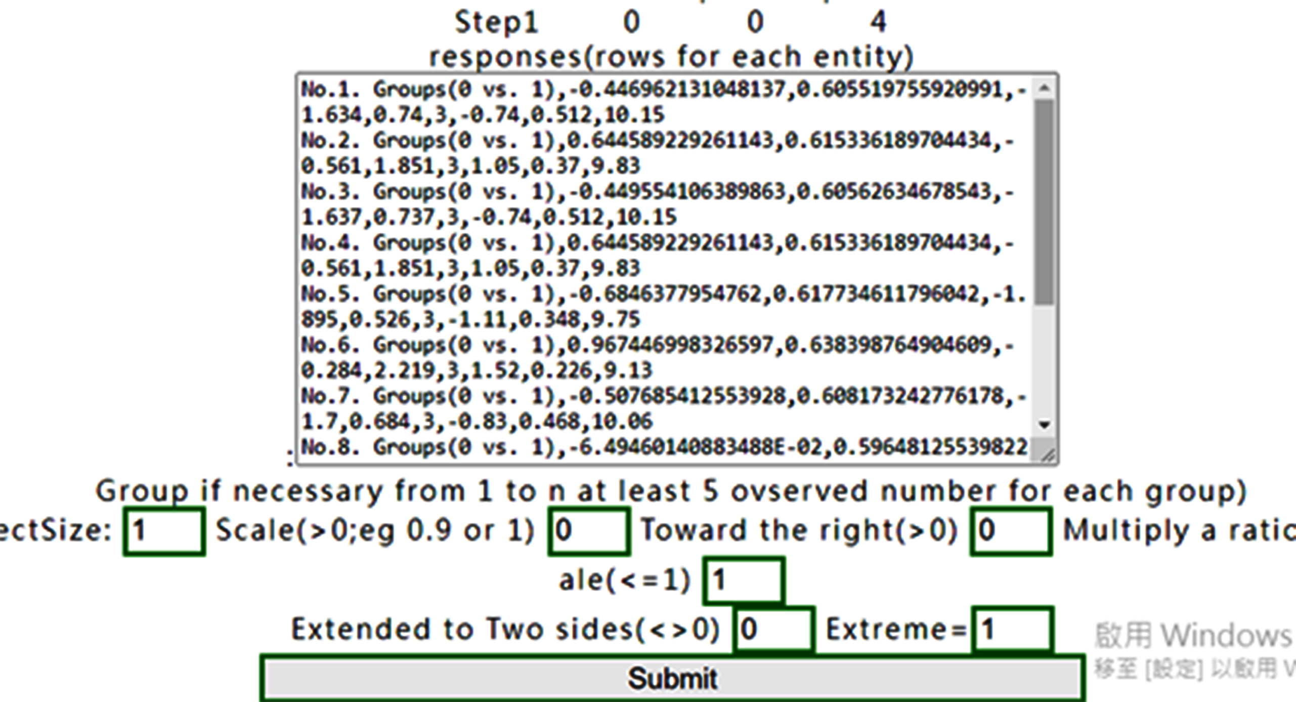
15.DIF:Table
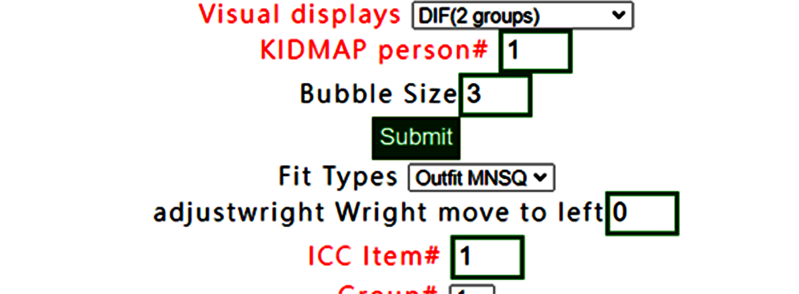
DIF(Table) has been selected(note. only for two group, 0 and 1 in group definition in RaschOnline).
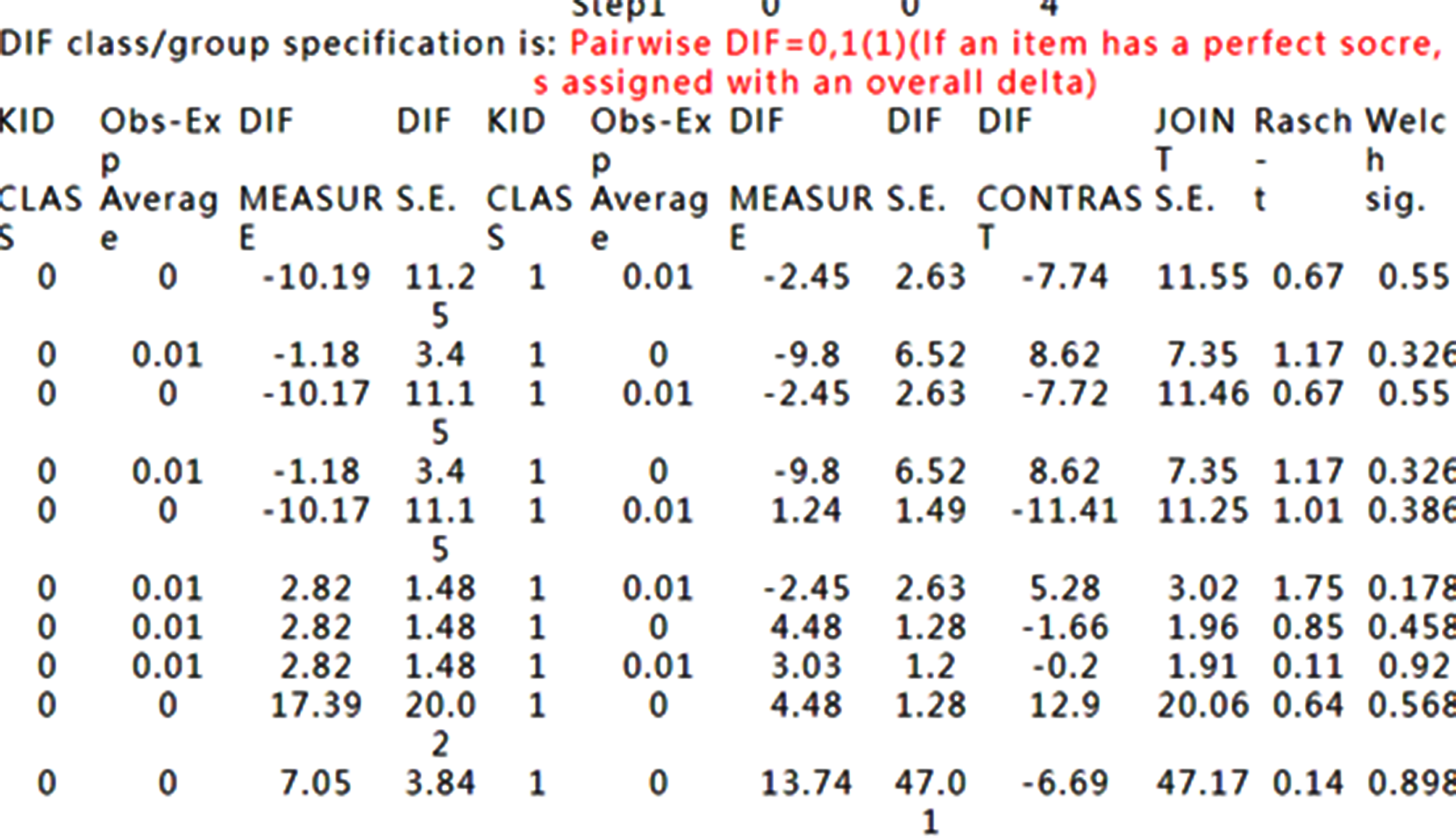
DIF Tables are shown accordingly.
How to interpret DIF Tables refers to Differential item functioning DIF pairwise at https://winsteps.com/winman/table30_1.htm
16.DIF:Graph
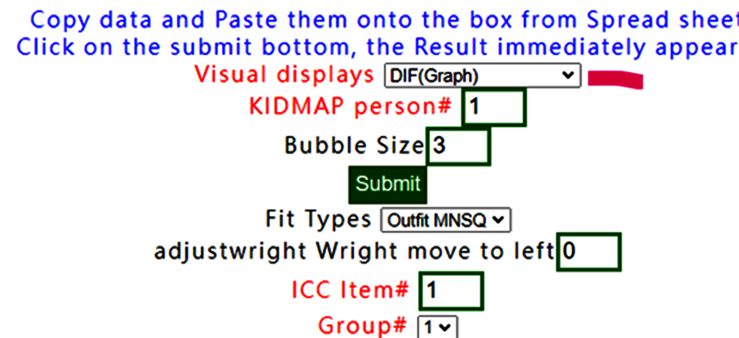
If DIF graph is selected, the graph using forest plot appears immediately on Google Maps after confirming the results below.
Confirm the contents
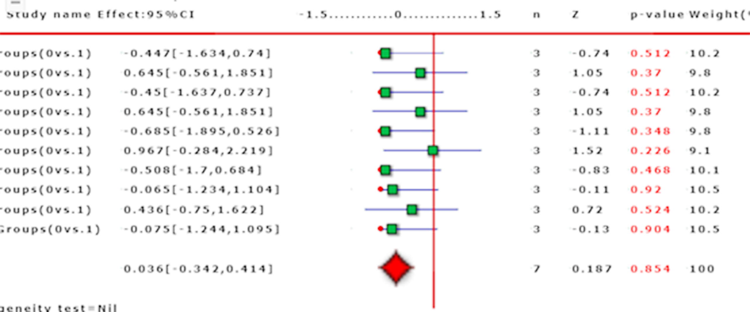
We can see that no DIF was found across all items in this dataset between groups 0 and 1.
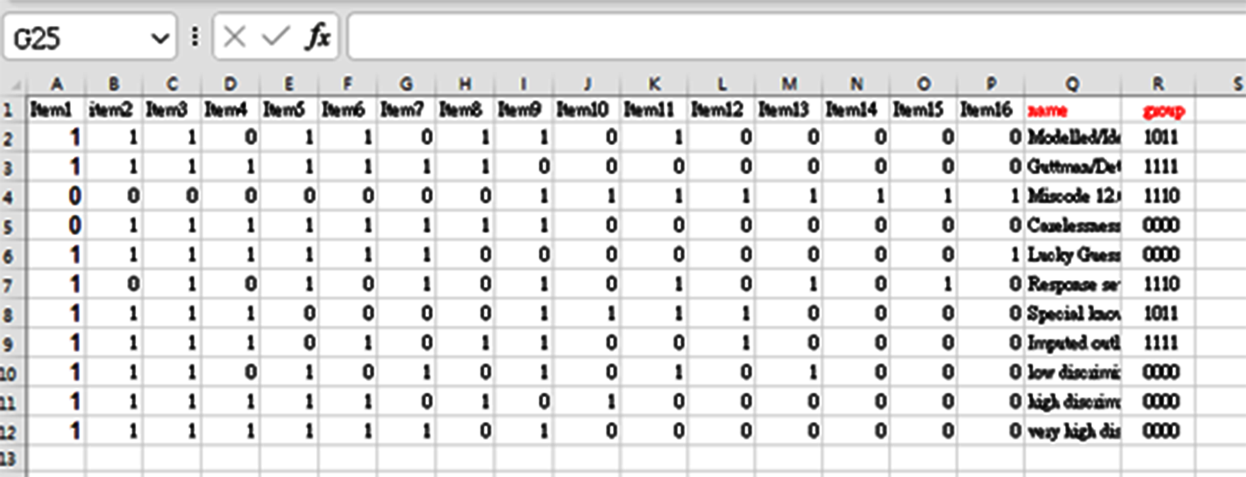
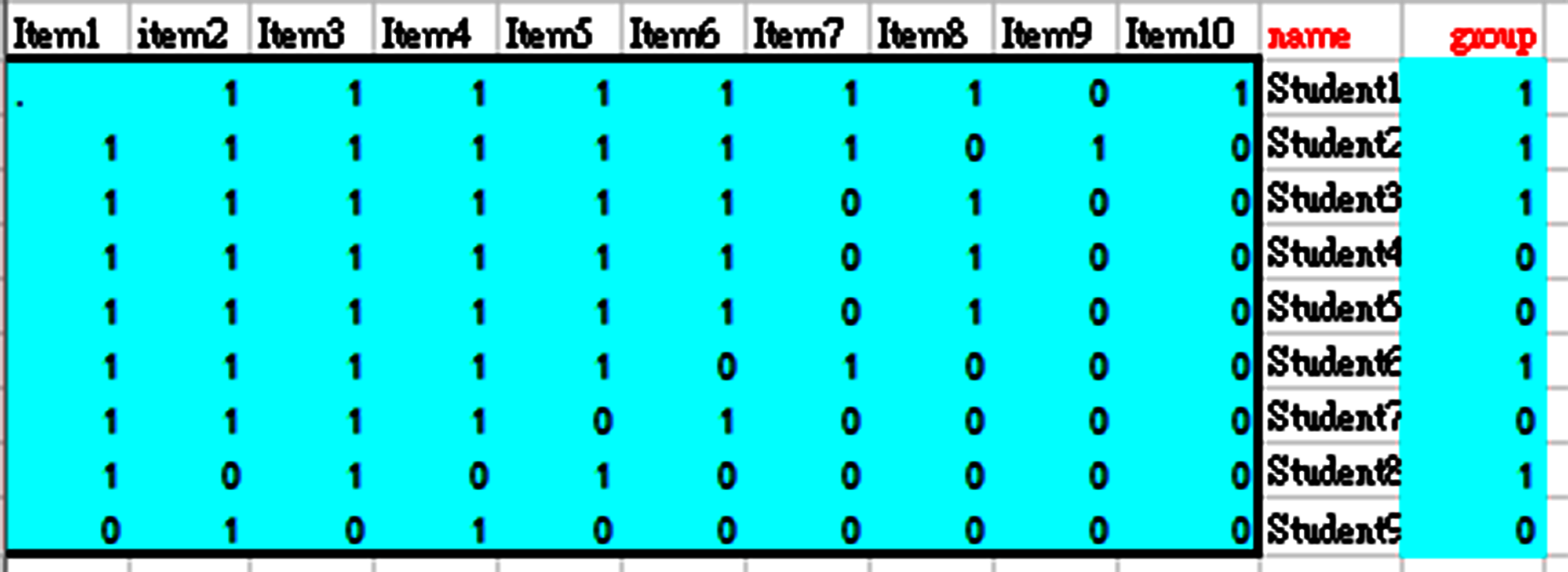
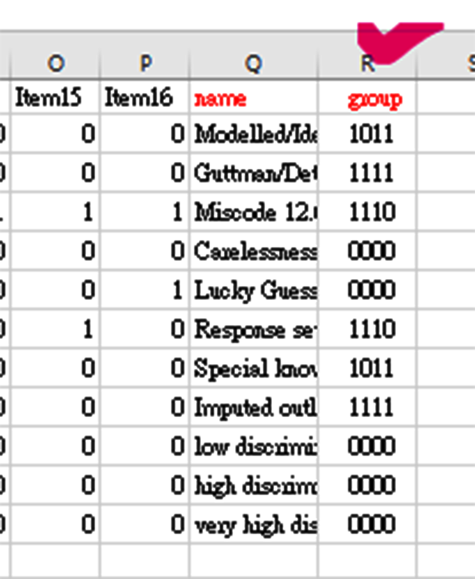
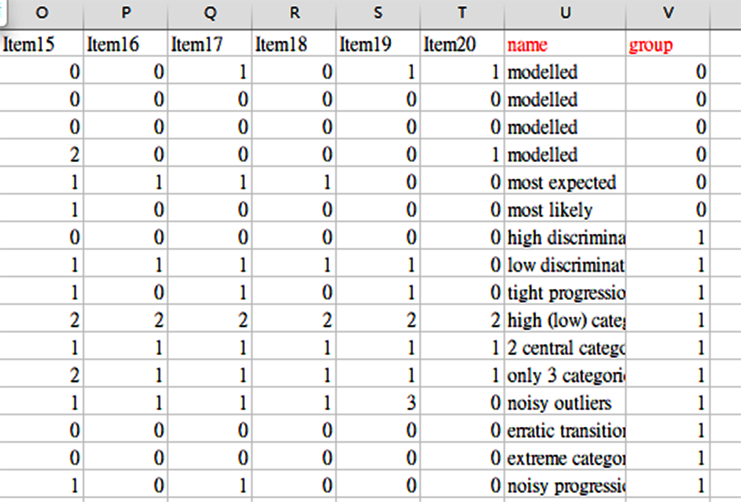
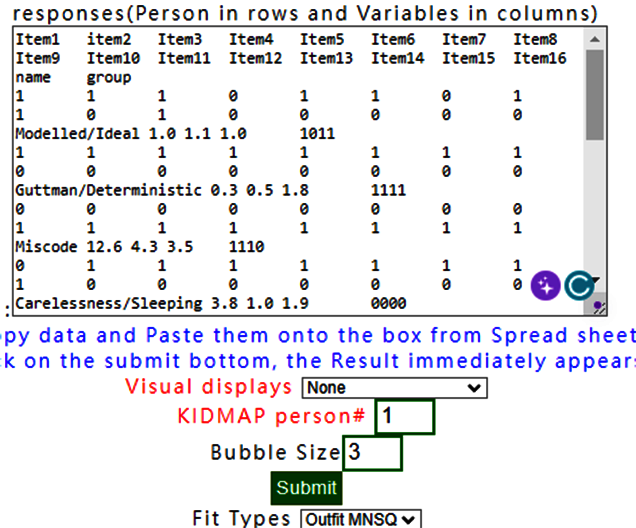
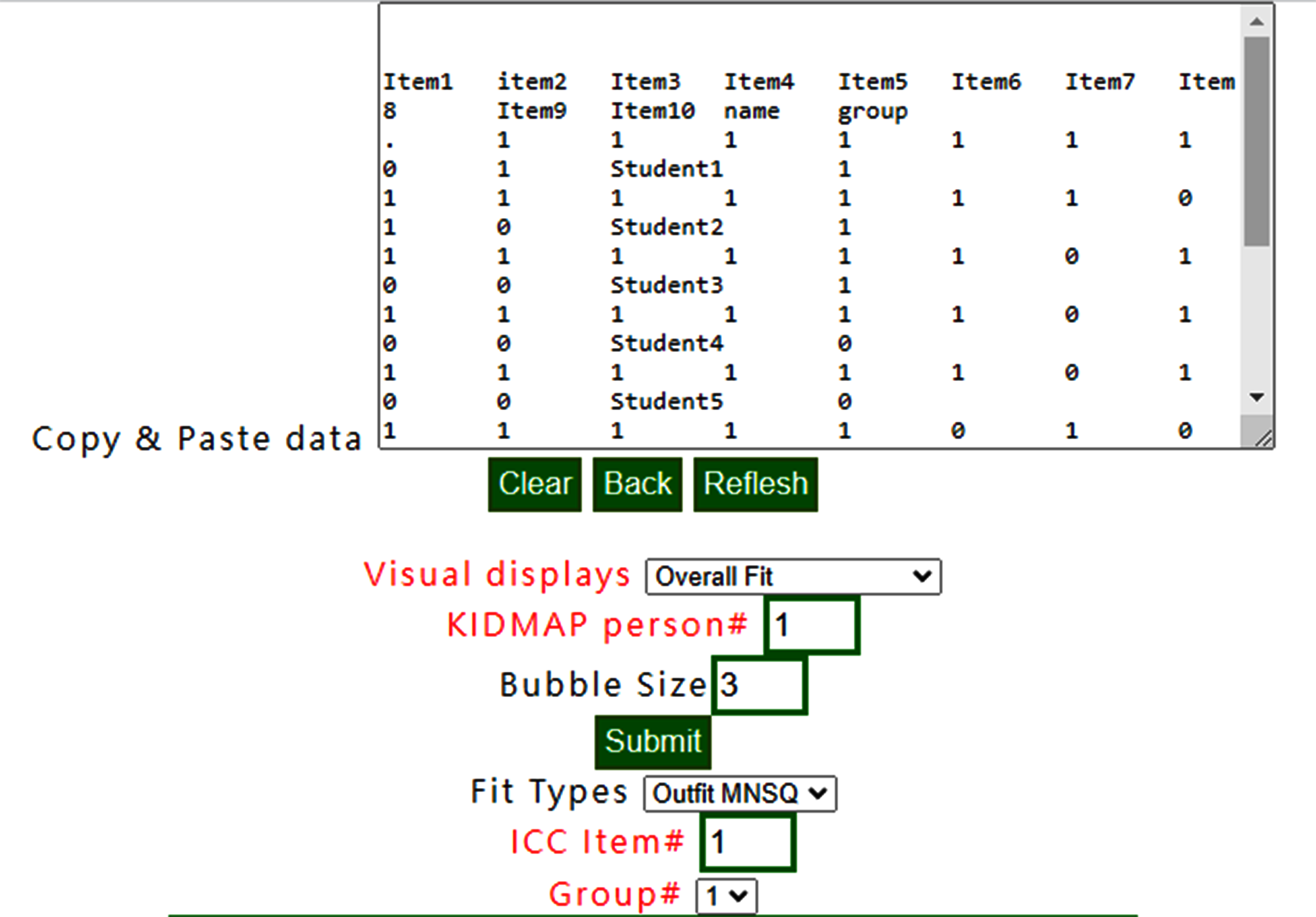
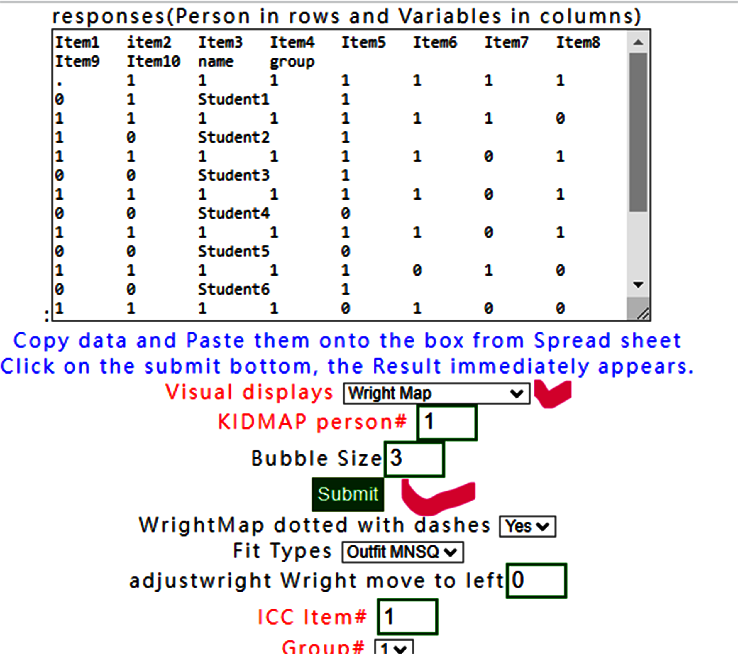
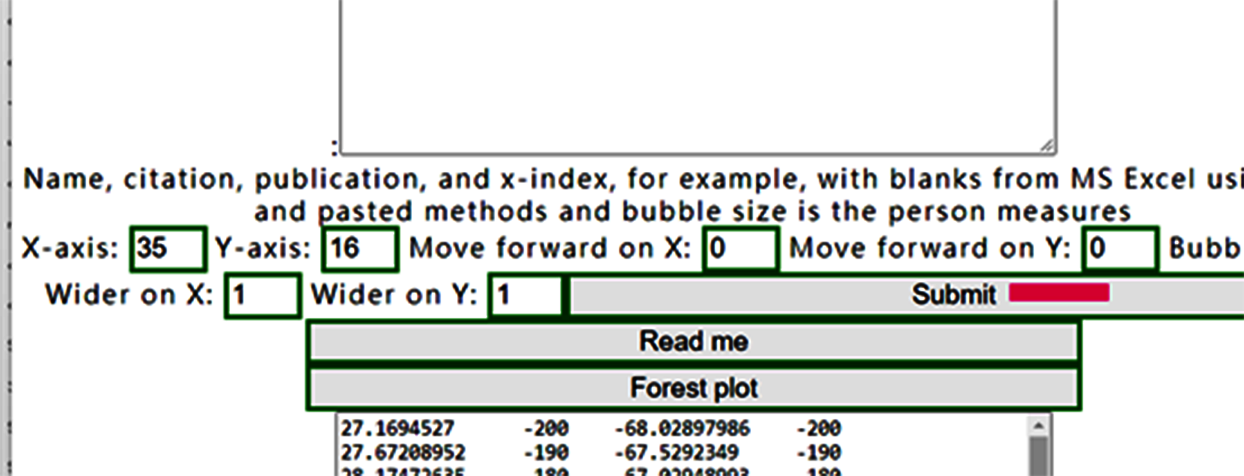
17.Copy & Paste
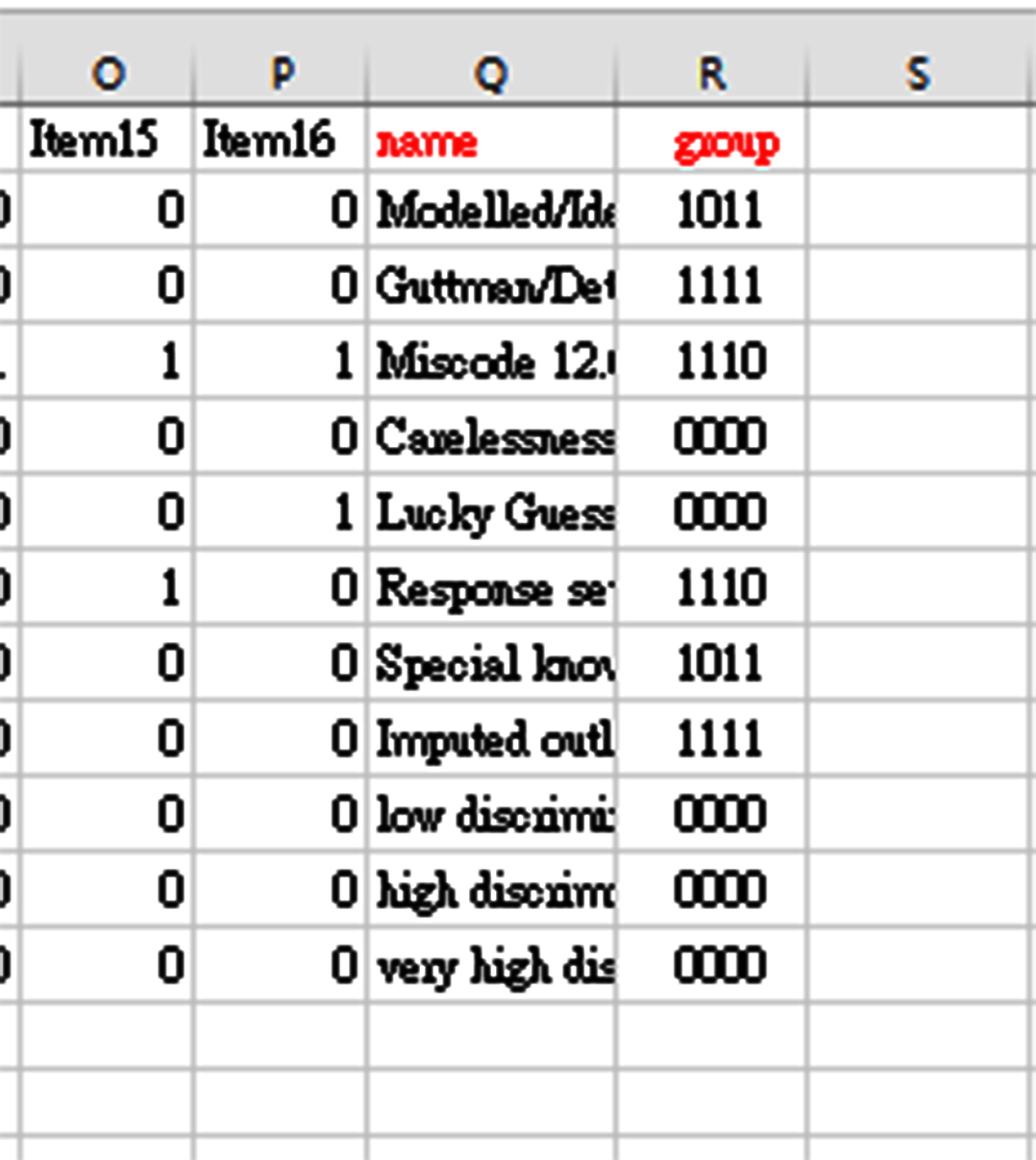
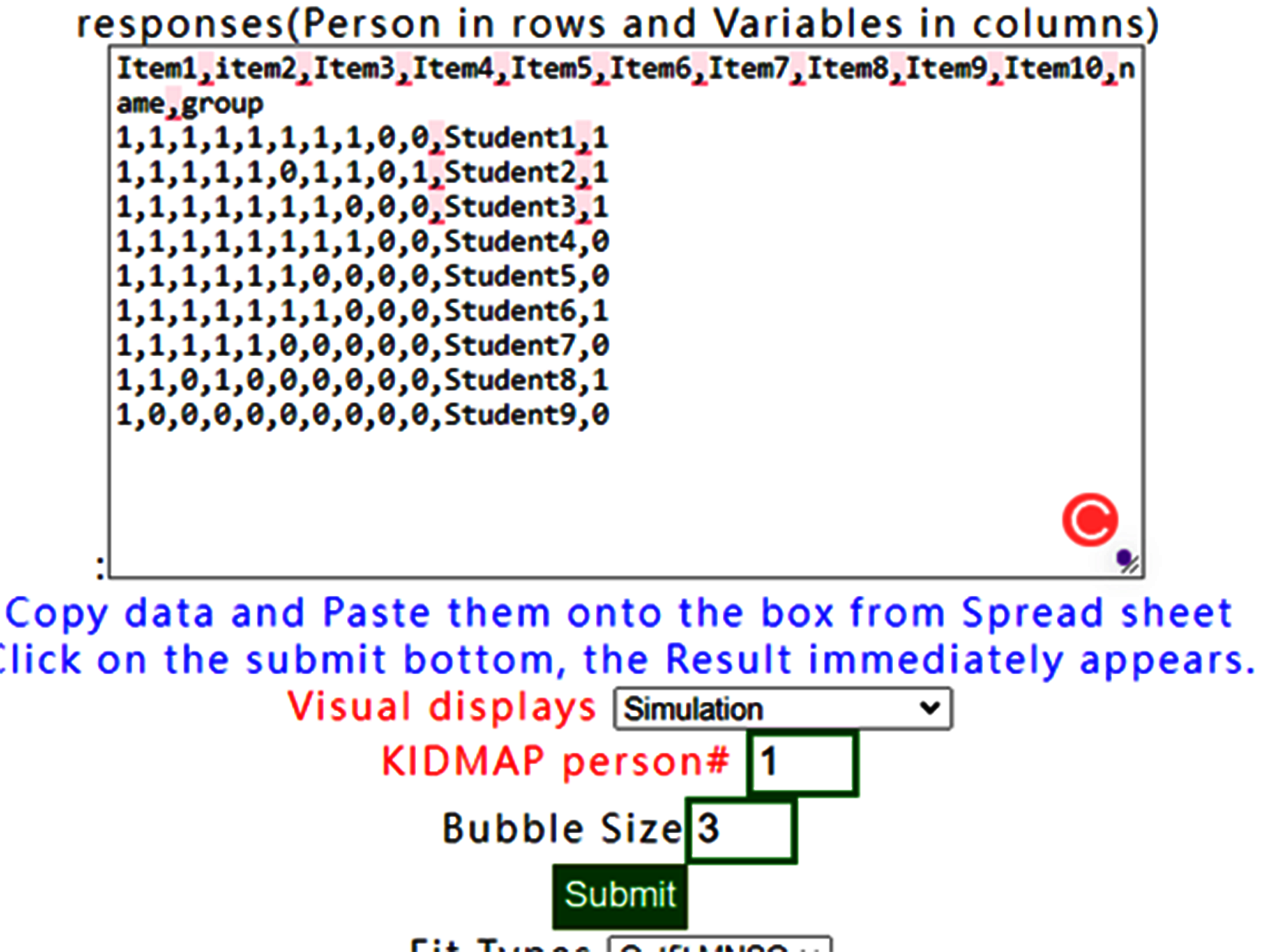
preparedness of Copy&paste data including head titles and last two with "name" and "group"
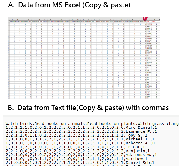
Paste data into the frame and then click on the submit bottom if no others selections necessary
Results displayed
ToTodisplay Wright Map.
To adjust bubble size to 1
Bubbles are adjusted to an appropriate layout.
To adjust the fit statistics with infit
Item infit MNSQs are displayed, different from those with Outfit MNSQ in the previous example.
If dash is selected.
the results are identical due to no step difficulties in the dichotomous scale as shown below:.
Otherwise, dashes are shown for RSM; see below.
6.Wright Map(Groups)
Wright Map with groups selected
More distributions in groups are displayed on the left-hand side.
Note. the summation of numbers in groups are identical to the total counts on the right-hand side.
7.KIDMAP
To select person number.
The one selected appears with a KIDMAP.
Another person is selected
Based on the person measure and fit statistics
The one with one item unexpected is found using KIDMAP
For person 2, we can see that item 8 in red bubble is unexpected(Zscore <-2.0) due to the easy item with incorrectness at the left-bottom side.
Another one with one item unexpected is found using KIDMAP.
For person 6, we can see that item 7 in red is harder but correct in the right-top side(Zscore>2.0)
If bubbles were selected with smaller size, the KIDMAP can be clear with expected and observed responses across items along with difficulties from top to bottom.
8.ICC_cat
The CATEGORY PROBABILITIES: MODES - Andrich thresholds at intersections with ICC shows item# 1 for all persons below:
We can see that only person 9 answers tem 1 incorrectly. Other persons answer item 1 with correctness on the success ogive cure for left-bottom to right-top corner.
Persons with higher ability are on the right-hand side. The bubble denoted by the vertical probability corresponds to the person ability.
Moving to the left on Google Maps, the ICC of item 1 is shown above. The red bubbles denote the observed responses by persons and the blue ones represent the expected responses by persons. The ChSQ statistics shown below, similar to the overall fit selected in the menu at the beginning.
Bubbles are colored by groups. We can see that only person 9 answers item 1 incorrectly. Other persons answer the item 1 with correctness on the success ogive cure for left-bottom to right-top corner.
Persons with higher ability are on the right-hand side. The bubble denoted by the vertical probability corresponds to the person ability.
To add lines linked to observed bubbles in ICC
The lines have been linked for observed responses of groups.
Why the ICC has six persons, but nine person in the dataset, which is the reason for the three persons have identical measures and make the bubble overlaid together.
9.Person fit plot(Outfit)
Select person fit plot with outfit MNSQ,
Outfit MNSQs are on the x-axis and person abilities are on the vertical y-axis. Bubbles are sized by person SE. In this case, we observed that all persons have outfit less than 2.0.
10.Person fit plot(Infit)
If Infit MNSQ is selected, the person fit plot is shown below:
Bubbles are sized by person SE and shown with infit MNSQ.
11.Measure/Outfit
Measure Outfit is selected.
The buffered form is generated. After confirming it, the plot is shown as below:
As the scatter plot shows the relationship between Outfit MNMS and person measure, three parts with colors are shown based on person strata.
12.Measure/Infit
Measure Infit is selected.
The buffered form is generated. After confirming it, the plot is shown as below:
As the scatter plot shows the relationship between Infit MNMS and person measure, three parts with colors are shown based on person strata.
13.Rawscore/Measure
When Rawscore/measure plot is selected using Kano diagram, the confirmation is shown below:
Confirm it and show the Kano diagram below:
We can see that all person measures are along with raw scores on the one-dimensional part in the diagram.
The correlation coefficient is 0.9758 shown below the plot.
14.Simulation data
The simulation data can be generated based on the reference at https://www.rasch.org/rmt/rmt213a.htm
The result below the website is the simulation data. We copy those data onto RaschOnline.
We can see that all person measures are along with raw scores on the one-dimensional part in the diagram.
Like this one above. If the visual display with None is selected, the results show all items fit to Rasch model when observing all infit/outfit MNSQ smaller than those in the original dataset.
See how well items fitting to the Rasch model
That is because the data fit Rasch model fairly well.
However, the two with extreme measures have larger standard errors in measures using Wright Map to display.
When the bubble of interest is clicked, the detailed information about the item appears on Google Maps.
15.DIF:Table
DIF(Table) has been selected(note. only for two group, 0 and 1 in group definition in RaschOnline).
DIF Tables are shown accordingly.
How to interpret DIF Tables refers to Differential item functioning DIF pairwise at https://winsteps.com/winman/table30_1.htm
16.DIF:Graph
If DIF graph is selected, the graph using forest plot appears immediately on Google Maps after confirming the results below.
Confirm the contents
We can see that no DIF was found across all items in this dataset between groups 0 and 1.
17.Copy & Paste
preparedness of Copy&paste data including head titles and last two with "name" and "group"
Paste data into the frame and then click on the submit bottom if no others selections necessary
Results displayed
More distributions in groups are displayed on the left-hand side. Note. the summation of numbers in groups are identical to the total counts on the right-hand side.
7.KIDMAP
To select person number.
The one selected appears with a KIDMAP.
Another person is selected
Based on the person measure and fit statistics
The one with one item unexpected is found using KIDMAP
For person 2, we can see that item 8 in red bubble is unexpected(Zscore <-2.0) due to the easy item with incorrectness at the left-bottom side.
Another one with one item unexpected is found using KIDMAP.
For person 6, we can see that item 7 in red is harder but correct in the right-top side(Zscore>2.0)
If bubbles were selected with smaller size, the KIDMAP can be clear with expected and observed responses across items along with difficulties from top to bottom.
8.ICC_cat
The CATEGORY PROBABILITIES: MODES - Andrich thresholds at intersections with ICC shows item# 1 for all persons below:
We can see that only person 9 answers tem 1 incorrectly. Other persons answer item 1 with correctness on the success ogive cure for left-bottom to right-top corner.
Persons with higher ability are on the right-hand side. The bubble denoted by the vertical probability corresponds to the person ability.
Moving to the left on Google Maps, the ICC of item 1 is shown above. The red bubbles denote the observed responses by persons and the blue ones represent the expected responses by persons. The ChSQ statistics shown below, similar to the overall fit selected in the menu at the beginning.
Bubbles are colored by groups. We can see that only person 9 answers item 1 incorrectly. Other persons answer the item 1 with correctness on the success ogive cure for left-bottom to right-top corner.
Persons with higher ability are on the right-hand side. The bubble denoted by the vertical probability corresponds to the person ability.
To add lines linked to observed bubbles in ICC
The lines have been linked for observed responses of groups.
Why the ICC has six persons, but nine person in the dataset, which is the reason for the three persons have identical measures and make the bubble overlaid together.
9.Person fit plot(Outfit)
Select person fit plot with outfit MNSQ,
Outfit MNSQs are on the x-axis and person abilities are on the vertical y-axis. Bubbles are sized by person SE. In this case, we observed that all persons have outfit less than 2.0.
10.Person fit plot(Infit)
If Infit MNSQ is selected, the person fit plot is shown below:
Bubbles are sized by person SE and shown with infit MNSQ.
11.Measure/Outfit
Measure Outfit is selected.
The buffered form is generated. After confirming it, the plot is shown as below:
As the scatter plot shows the relationship between Outfit MNMS and person measure, three parts with colors are shown based on person strata.
12.Measure/Infit
Measure Infit is selected.
The buffered form is generated. After confirming it, the plot is shown as below:
As the scatter plot shows the relationship between Infit MNMS and person measure, three parts with colors are shown based on person strata.
13.Rawscore/Measure
When Rawscore/measure plot is selected using Kano diagram, the confirmation is shown below:
Confirm it and show the Kano diagram below:
We can see that all person measures are along with raw scores on the one-dimensional part in the diagram.
The correlation coefficient is 0.9758 shown below the plot.
14.Simulation data
The simulation data can be generated based on the reference at https://www.rasch.org/rmt/rmt213a.htm
The result below the website is the simulation data. We copy those data onto RaschOnline.
We can see that all person measures are along with raw scores on the one-dimensional part in the diagram.
Like this one above. If the visual display with None is selected, the results show all items fit to Rasch model when observing all infit/outfit MNSQ smaller than those in the original dataset.
See how well items fitting to the Rasch model
That is because the data fit Rasch model fairly well.
However, the two with extreme measures have larger standard errors in measures using Wright Map to display.
When the bubble of interest is clicked, the detailed information about the item appears on Google Maps.
15.DIF:Table
DIF(Table) has been selected(note. only for two group, 0 and 1 in group definition in RaschOnline).
DIF Tables are shown accordingly.
How to interpret DIF Tables refers to Differential item functioning DIF pairwise at https://winsteps.com/winman/table30_1.htm
16.DIF:Graph
If DIF graph is selected, the graph using forest plot appears immediately on Google Maps after confirming the results below.
Confirm the contents
We can see that no DIF was found across all items in this dataset between groups 0 and 1.
17.Copy & Paste
preparedness of Copy&paste data including head titles and last two with "name" and "group"
Paste data into the frame and then click on the submit bottom if no others selections necessary
Results displayed
The CATEGORY PROBABILITIES: MODES - Andrich thresholds at intersections with ICC shows item# 1 for all persons below:
We can see that only person 9 answers tem 1 incorrectly. Other persons answer item 1 with correctness on the success ogive cure for left-bottom to right-top corner.
Persons with higher ability are on the right-hand side. The bubble denoted by the vertical probability corresponds to the person ability.
Moving to the left on Google Maps, the ICC of item 1 is shown above. The red bubbles denote the observed responses by persons and the blue ones represent the expected responses by persons. The ChSQ statistics shown below, similar to the overall fit selected in the menu at the beginning.
Bubbles are colored by groups. We can see that only person 9 answers item 1 incorrectly. Other persons answer the item 1 with correctness on the success ogive cure for left-bottom to right-top corner.
Persons with higher ability are on the right-hand side. The bubble denoted by the vertical probability corresponds to the person ability.
To add lines linked to observed bubbles in ICC
The lines have been linked for observed responses of groups.
Persons with higher ability are on the right-hand side. The bubble denoted by the vertical probability corresponds to the person ability.
Moving to the left on Google Maps, the ICC of item 1 is shown above. The red bubbles denote the observed responses by persons and the blue ones represent the expected responses by persons. The ChSQ statistics shown below, similar to the overall fit selected in the menu at the beginning.
Persons with higher ability are on the right-hand side. The bubble denoted by the vertical probability corresponds to the person ability.
To add lines linked to observed bubbles in ICC
Why the ICC has six persons, but nine person in the dataset, which is the reason for the three persons have identical measures and make the bubble overlaid together.
9.Person fit plot(Outfit)
Select person fit plot with outfit MNSQ,
Outfit MNSQs are on the x-axis and person abilities are on the vertical y-axis. Bubbles are sized by person SE. In this case, we observed that all persons have outfit less than 2.0.
10.Person fit plot(Infit)
If Infit MNSQ is selected, the person fit plot is shown below:
Bubbles are sized by person SE and shown with infit MNSQ.
11.Measure/Outfit
Measure Outfit is selected.
The buffered form is generated. After confirming it, the plot is shown as below:
As the scatter plot shows the relationship between Outfit MNMS and person measure, three parts with colors are shown based on person strata.
12.Measure/Infit
Measure Infit is selected.
The buffered form is generated. After confirming it, the plot is shown as below:
As the scatter plot shows the relationship between Infit MNMS and person measure, three parts with colors are shown based on person strata.
13.Rawscore/Measure
When Rawscore/measure plot is selected using Kano diagram, the confirmation is shown below:
Confirm it and show the Kano diagram below:
We can see that all person measures are along with raw scores on the one-dimensional part in the diagram.
The correlation coefficient is 0.9758 shown below the plot.
14.Simulation data
The simulation data can be generated based on the reference at https://www.rasch.org/rmt/rmt213a.htm
The result below the website is the simulation data. We copy those data onto RaschOnline.
We can see that all person measures are along with raw scores on the one-dimensional part in the diagram.
Like this one above. If the visual display with None is selected, the results show all items fit to Rasch model when observing all infit/outfit MNSQ smaller than those in the original dataset.
See how well items fitting to the Rasch model
That is because the data fit Rasch model fairly well.
However, the two with extreme measures have larger standard errors in measures using Wright Map to display.
When the bubble of interest is clicked, the detailed information about the item appears on Google Maps.
15.DIF:Table
DIF(Table) has been selected(note. only for two group, 0 and 1 in group definition in RaschOnline).
DIF Tables are shown accordingly.
How to interpret DIF Tables refers to Differential item functioning DIF pairwise at https://winsteps.com/winman/table30_1.htm
16.DIF:Graph
If DIF graph is selected, the graph using forest plot appears immediately on Google Maps after confirming the results below.
Confirm the contents
We can see that no DIF was found across all items in this dataset between groups 0 and 1.
17.Copy & Paste
preparedness of Copy&paste data including head titles and last two with "name" and "group"
Paste data into the frame and then click on the submit bottom if no others selections necessary
Results displayed
The buffered form is generated. After confirming it, the plot is shown as below:
As the scatter plot shows the relationship between Outfit MNMS and person measure, three parts with colors are shown based on person strata.
12.Measure/Infit
Measure Infit is selected.
The buffered form is generated. After confirming it, the plot is shown as below:
As the scatter plot shows the relationship between Infit MNMS and person measure, three parts with colors are shown based on person strata.
13.Rawscore/Measure
When Rawscore/measure plot is selected using Kano diagram, the confirmation is shown below:
Confirm it and show the Kano diagram below:
We can see that all person measures are along with raw scores on the one-dimensional part in the diagram.
The correlation coefficient is 0.9758 shown below the plot.
14.Simulation data
The simulation data can be generated based on the reference at https://www.rasch.org/rmt/rmt213a.htm
The result below the website is the simulation data. We copy those data onto RaschOnline.
We can see that all person measures are along with raw scores on the one-dimensional part in the diagram.
Like this one above. If the visual display with None is selected, the results show all items fit to Rasch model when observing all infit/outfit MNSQ smaller than those in the original dataset.
See how well items fitting to the Rasch model
That is because the data fit Rasch model fairly well.
However, the two with extreme measures have larger standard errors in measures using Wright Map to display.
When the bubble of interest is clicked, the detailed information about the item appears on Google Maps.
15.DIF:Table
DIF(Table) has been selected(note. only for two group, 0 and 1 in group definition in RaschOnline).
DIF Tables are shown accordingly.
How to interpret DIF Tables refers to Differential item functioning DIF pairwise at https://winsteps.com/winman/table30_1.htm
16.DIF:Graph
If DIF graph is selected, the graph using forest plot appears immediately on Google Maps after confirming the results below.
Confirm the contents
We can see that no DIF was found across all items in this dataset between groups 0 and 1.
17.Copy & Paste
preparedness of Copy&paste data including head titles and last two with "name" and "group"
Paste data into the frame and then click on the submit bottom if no others selections necessary
Results displayed
We can see that all person measures are along with raw scores on the one-dimensional part in the diagram. Like this one above. If the visual display with None is selected, the results show all items fit to Rasch model when observing all infit/outfit MNSQ smaller than those in the original dataset.
See how well items fitting to the Rasch model
That is because the data fit Rasch model fairly well.
However, the two with extreme measures have larger standard errors in measures using Wright Map to display.
When the bubble of interest is clicked, the detailed information about the item appears on Google Maps.
15.DIF:Table
DIF(Table) has been selected(note. only for two group, 0 and 1 in group definition in RaschOnline).
DIF Tables are shown accordingly.
How to interpret DIF Tables refers to Differential item functioning DIF pairwise at https://winsteps.com/winman/table30_1.htm
16.DIF:Graph
If DIF graph is selected, the graph using forest plot appears immediately on Google Maps after confirming the results below.
Confirm the contents
We can see that no DIF was found across all items in this dataset between groups 0 and 1.
17.Copy & Paste
preparedness of Copy&paste data including head titles and last two with "name" and "group"
Paste data into the frame and then click on the submit bottom if no others selections necessary
Results displayed